Global RBF engine
The Radial Basis Function (RBF) engine is an interpolation method used in geological modelling. It estimates values such as lithology, density, or elevation at unsampled locations by smoothly interpolating between known data points using radial basis functions. Common applications include generating geological contact surfaces, fault planes, intrusive boundaries, and numerical grade cut-off models.
The GeologyCoreRBF engine provides several settings to control how surfaces are interpolated and shaped. Below are the available parameters:
Interpolant function
This is the RBF kernel function used in the interpolation. There are two available options:
-
Linear
-
Spheroidal
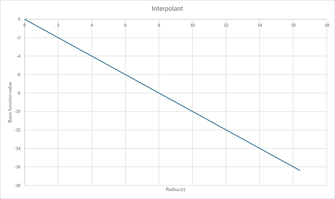
Linear interpolant
The Linear interpolant can be thought of as stretching a flexible sheet through your data points. The surface adjusts smoothly to your inputs but keeps things simple with no "cut-off" for how far each point influences the model.
This method is ideal for broad, continuous features or when you are in the early stages of modelling.
When to use it:
-
Your surfaces are large and simple (e.g. flat or gently folded).
-
You have few data points, or they’re widely spaced.
-
You want a quick first pass before refining your model.
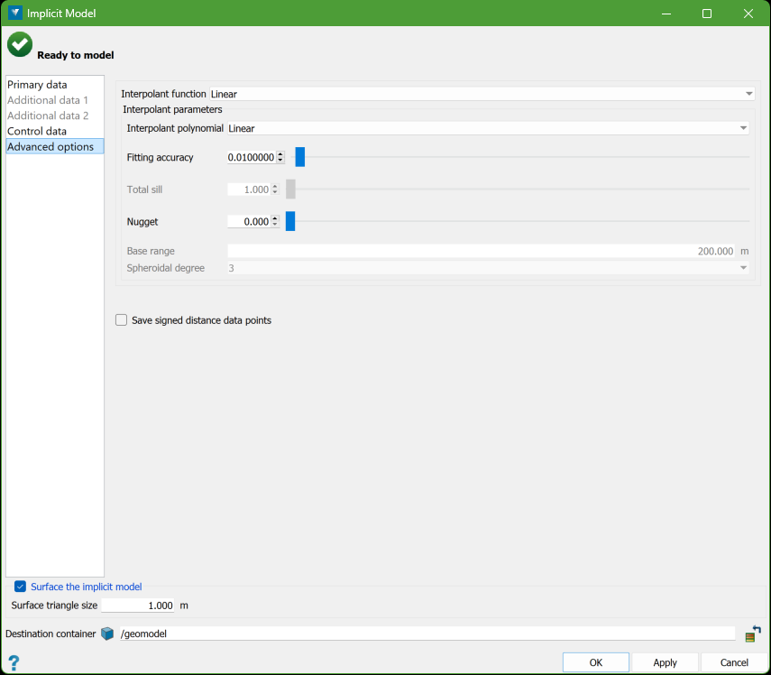
Interpolant parameters
Interpolant Polynomial (Drift)
Adds a background value to the interpolant:
-
Constant: Adds a fixed background value to the model, helping the interpolant stay stable away from data.
-
Linear: Allows the interpolant to undulate away from data, shaped by the overall distribution of the data.
Fitting Accuracy
Controls how precise the model needs to be when solving. It guarantees that evaluating the RBF at the input source points will reproduce the input values within this tolerance.
-
Lower values = better fit to data but longer computation time.
-
Higher values = faster results but less precision.
Nugget
Smooths the result by reducing how strictly the model honours each point.
-
A small nugget makes the model pass almost exactly through your inputs.
-
A larger nugget lets the model "soften" the fit, which can be useful if your data is noisy.
Spheroidal interpolant
The Spheroidal interpolant gives you more control over how far a point’s influence spreads and how quickly that influence fades.
Think of each point as sending out a "signal" that weakens with distance. You define how far the signal travels (range), how strong it is (sill), and how quickly it drops off (degree).
This method works well for detailed, localised features like mineral lenses or grade cut-offs.
When to use it:
-
Your data shows tight, local variation or strong zonation.
-
You want to mimic behaviour similar to variogram-based models.
-
You need more control over continuity and influence range.
Interpolant parameters
Interpolant Polynomial (Drift)
Adds a background value to the interpolant:
-
None: No added background value, meaning the interpolant tends to zero away from data.
-
Constant: Adds a fixed background value to the model, helping the interpolant stay stable away from data.
-
Linear: Allows the interpolant to undulate away from data, shaped by the overall distribution of the data.
Fitting Accuracy
Controls how precise the model needs to be when solving. It guarantees that evaluating the RBF at the input source points will reproduce the input values within this tolerance.
-
Lower values = better fit to data but longer computation time.
-
Higher values = faster results but less precision.
Nugget
Similar to Linear drift: it reduces overfitting to noisy data.
-
A small nugget makes the model pass almost exactly through your inputs.
-
A larger nugget lets the model "soften" the fit, which can be useful if your data is noisy.
The higher the nugget value, the less influence anomalous measurements have. Anomalous measurements could come from outlying samples or errors.
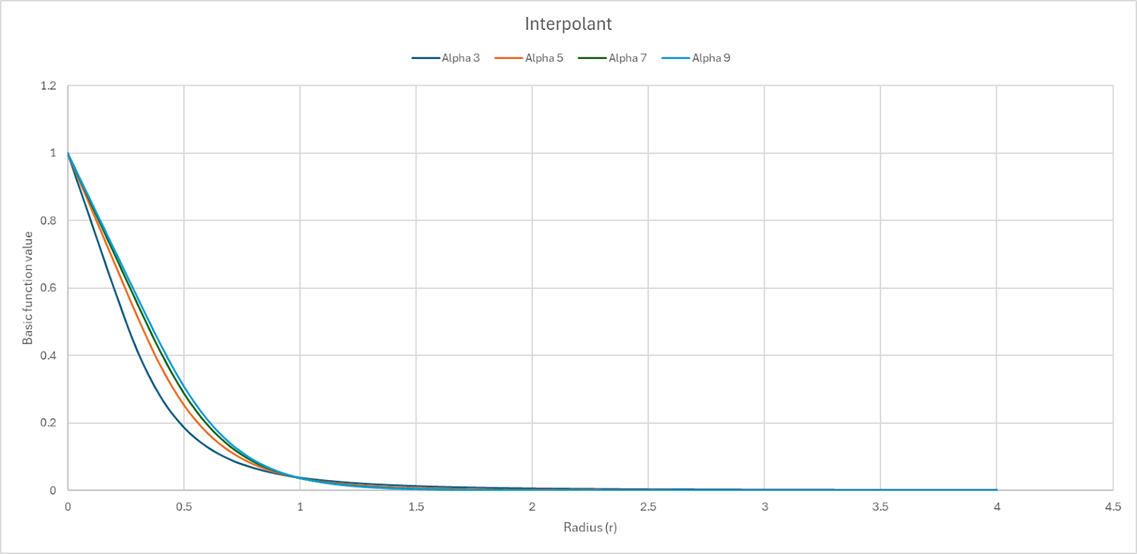
Spheroidal Degree (Alpha)
This controls the shape of the interpolant function and how quickly it tends towards zero.
-
A higher degree value gives more weight to points farther away.
-
A lower degree value places more weight on points closer by.