Sequential Indicator

Use this option to assist in determining geological boundaries where they are not well defined.

Instructions

On the Block menu, point to Simulation, and then click Sequential Indicator.

Simulation Parameters

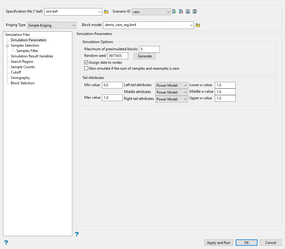
Use this pane to define the specification file, scenario ID, kriging method, and block model. You can also select which simulation options to use, and set the tail attributes.

Follow these steps:

Enter a name for the Estimation file, or select it from the drop-down list. The drop-down list displays all files found in the current working directory that have the (.bef) extension. Click the Browse icon to select a file from another location.
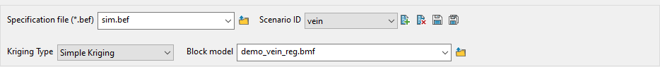
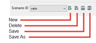
Select a Scenario ID. To create a new ID, click the New icon as shown below, and provide a unique name for the current panel settings. Up to nine separate IDs can be created for each BEF file.
Select the Kriging type to use when establishing the conditional distribution parameters.

The following methods are available:
- Use simple kriging
- Use simple kriging with local mean
- Ordinary kriging
Note: A block model variable storing the local mean must exist to use simple kriging with local mean. You can select the variable using the drop-down list in the table on the Cutoff pane.
Select the Block model from the drop-down list. Click the Browse icon to select a file from another location.

Enter the maximum number of previously estimated blocks to use in the field Maximum of presimulated blocks. As stochastic simulation proceeds, it collects samples from previously estimated blocks and from sample data.
Enter the Random seed number. Click the Generate button if you want Vulcan to produce the seed number.

The random numbers used by Vulcan are actually pseudo-random numbers that can be reproduced by starting with the same initial conditions. The random number seed controls which sequence of random numbers Vulcan uses. By using the same random number seed, previous results can be reproduced. Hence by using different random number seeds, different simulations are produced. Each stochastic simulation run will only produce one possible set of values in the block model. It is desirable to run several different stochastic simulations with the same parameters, but different random seeds, to see the possible variability in the simulated values.

Note: To select values for the simulation, Vulcan picks random values from a distribution. To calculate a distribution, Vulcan performs the equivalent of simple indicator kriging.
Select Assign data to nodes if you want sample locations to be slightly modified by considering them to be at the location of the closest node within the block model. This allows for faster simulation results, however, some samples could be lost as when more than one sample is contained in a block, only the closest is assigned and the other is discarded for simulation. Discarded samples are still used to build the global distribution and Gaussian transformation if required.
Select Non simulate if the sum of samples and resamples is zero if you do not want to include the block in the simulation if there are no samples or presimulated blocks within the range of the search. The block will be assigned a the default value
Enter the Minimum value to be used in the distribution. This value should be less than the smallest cut-off.
Enter the Maximum value to be used in the distribution.
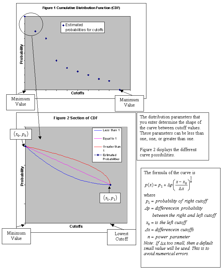
Select a model for each section of tail attribute using the drop-down lists.

Power model for left tail - This describes the shape of a curve from the Minimum data value to the lowest cut-off. If this value is less than 1, then the distribution is skewed towards the minimum data value. If it is greater than 1, then the distribution is skewed towards the lowest cut-off. If it is equal to 1, then the distribution is flat from the minimum data value to the lowest cut-off.

Power model for right tail - This option gives a distribution with a maximum data value. The maximum data value should be larger than the highest cut-off. The power for the right tail curve controls the shape of the distribution above the highest cut-off. If the power is less than 1, then the distribution is skewed towards the highest cut-off. If the power is greater than 1, then the distribution is skewed towards the maximum data value.

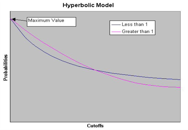
Hyperbolic model for right tail - This option gives a distribution with no maximum. If the power is greater than 1, then the distribution contains more values closer to the highest cut-off and less higher values. Whereas if the power is less than 1, then the distribution contains less values closer to the highest cut-off, but more higher values. The hyperbolic model right tail option always allows for the possibility of arbitrarily large simulated values.
Enter the power for the interpolation curves in the fields labelled Lower w value, Middle w value, and Upper w value. This describes the shape of the curve between cut-off values. If it is less than 1, then the distribution is skewed towards the left. If it is greater than 1, then it is skewed towards the right between cut-offs. If it is equal to 1, then the distribution is flat between cut-offs.

Samples Selection

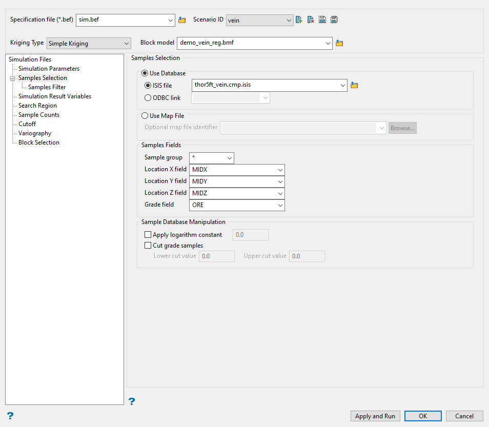
Use this pane to define the source of your samples. You can use an Isis database or a map file.

Follow these steps:

Select either a database or map file as your sample source.
- To select a database, enable the option ISIS file, then select the file from the drop-down list. Click folder icon to select a file from another location.
  
  You can also select an ODBC link for database files found on site servers.
- To select a map file, enable the option labelled Use Map File, then select the file from the drop-down list. Click the Browse button to select a file from another location.
Map the correct fields by filling out the Samples Fields information.
1. Sample group - Enter the name of the groups (database keys) to be loaded in the field. Wildcards (* multi-character wildcard and % single character wildcard) may be used to select multiple groups. Multiple groups only apply to Isis databases (ASCII map files consist of one group).
2. Select the names of the fields containing the X, Y, and Z coordinates in the Location fields.
3. Select the name for the variable containing the Grade values.
Select one or both of the Sample database manipulation options to apply to your data. This is not required.
- Apply logarithm - Select this option to apply the base logarithm function to all sample values.
  
  Note: All original sample values must be positive for the logarithm to be defined. The specified logarithm constant is added to the calculated logarithm.
- Cut grade samples - Select this option to apply cut-offs to the grades used in the estimation. Specify a lower grade cut value (grades lower than this value are set to this value) and an upper grade cut value (grades above this value are set to this value).

Samples Filter

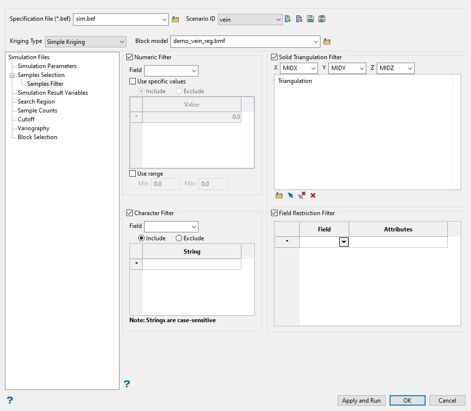
Use this pane to include any restrictions to your data by using the four specialised filters.

Follow these steps:

Include any restrictions to your data by using the four specialised filters.
Select using Numeric tag
Use this filter to limit a numeric variable by only using specific values, ignoring specific values, or setting a range of values that can be used.

Follow these steps:
1. Enable this pane by selecting Sample Selection Using a Numeric tag.
2. Select the numeric field from the drop-down list.
3. Select Use specific numeric values to limit the values to only those listed in the table.
4. Select Ignore certain numeric values to create a list of values that will be ignored.
5. Select Use a numeric range to use all values found between a minimum and maximum threshold.
Note: You can use more than one filter. However, keep in mind that all conditions must be met for a value to be used.
Select using Character tag
Use this filter to limit a character variable by only using specific values or ignoring specific values.

Follow these steps:
1. Enable this pane by selecting Sample Selection Using a Character tag.
2. Select the Character field from the drop-down list.
3. Select Use specific character values to limit the values to only those listed in the table.
4. Select Ignore certain character values to create a list of values that will be ignored.
Note: You can use more than one filter. However, keep in mind that all conditions must be met for a value to be used.
Select using Solid triangulations
Use this filter to limit the samples by one or more triangulations.

Follow these steps:
1. Enable this pane by selecting Select using solid triangulations.
2. Add triangulations to the list by clicking the Browse or Screen Pick button.
  
  Clicking Browse will cause an Explorer panel to display.
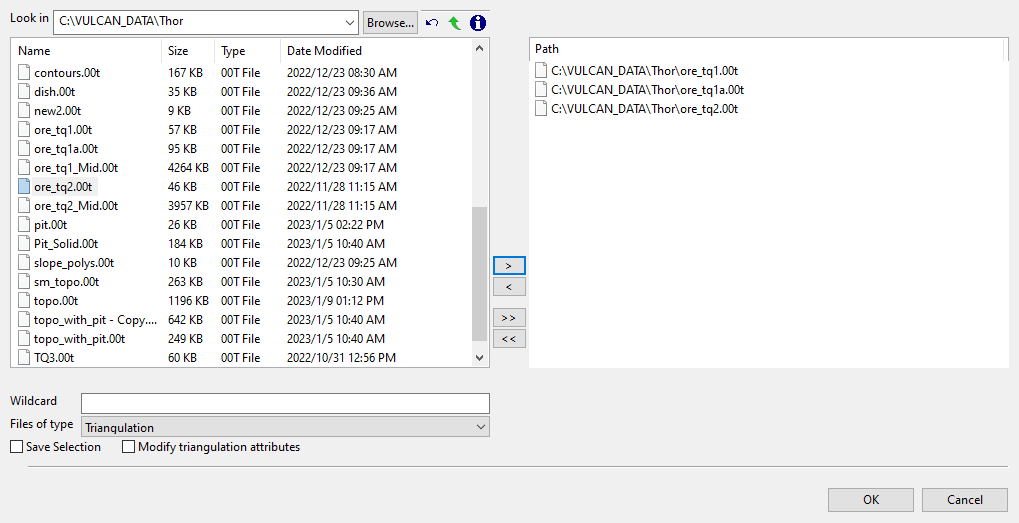
  Select Triangulation(s) panel
  
  Select the desired triangulation file(s) from the file list, which shows all available files in the current working directory. You can select files from a different location by clicking Browse..., or use the buttons to go to the last folder visited, go up one level, or change the way details are viewed in the panel, respectively.
  
  To highlight multiple list items at once, use the left mouse option in combination with the Shiftkey (this is for items that are adjacent in the list; for non-adjacent items, use the Ctrlkey and the left mouse option).
  
  Tip
  To filter file names using wildcard characters, type in a pattern in the Wildcard field using * for a multi-character and ? for a single-character wildcard.
  
  If you would like to use a previously created selection file (.sel) containing a list of desired triangulation files to load, choose Selection Files (*.sel) from the Files of type drop-down list.
  
  Move the items to the selection list on the right side of the panel.
  
  Click the button to move the highlighted items to the selection list on the right.
  
  Click the button to remove the highlighted items from the selection list on the right.
  
  Click the button to move all items to the selection list on the right.
  
  Click the button to remove all items from the selection list on the right.
  
  Select the Save Selection checkbox if you want to save the selection list (the right side of the panel), to a nominated selection file (.sel). Once this panel has been completed, a panel displays to save the selection file. Choose a selection file from the File Explorer to store the triangulation selection list to and click Save. To create a new file, enter the file name.
  
  Click OK to load the list of selected triangulations. Alternatively, click Cancel to close the panel without loading the selected triangulations.
3. Removing triangulations from the list by clicking the Clear Selected or Clear All button.
Select using Field restrictions
Use this filter to limit the samples to those with fields that match certain selection criteria.

Follow these steps:
1. Enable this pane by selecting Select selection using field restriction.
2. Select the field from the drop-down list in the Field column.
3. Enter the conditions that must be met in the Attributes column.
  
  Include spaces only if spaces are included in the desired field values.
  
  When entering a range, always enter the smallest number specified before the largest number.
  
  -792&-720 since -792 is smaller than -720. This range is evaluated as -792.0 ≤ VALUE < -720.0.
  
  Note: You can enter more than one condition. However, keep in mind that all conditions must be met for a value to be used.

Simulation Result Variables

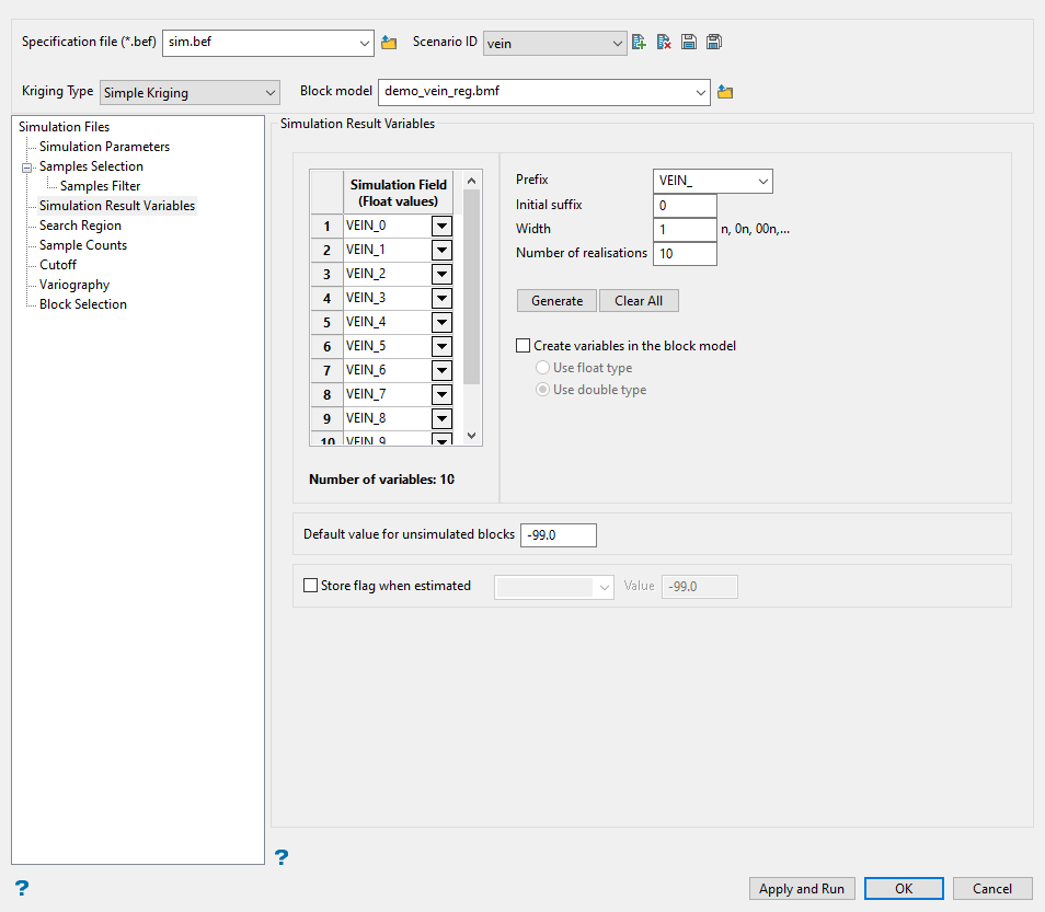
Use this pane to manually select the variable that will be used to store each one of the realisations. In addition, an automatic tool can be used to create the necessary variables.

Follow these steps:

Enter the Prefix for the variable name. You can use one from the drop-down list or enter your own.
Enter the starting number in the sequence in the Initial suffix field.
Enter the minimum number of characters that can be used to represent a number in the Width field.

Example: A prefix of simwith an initial suffix of 1and a width of 3would result in sim001as the first simulation field.
Enter the Number of realisations you want to run.
Use the Generate button to populate the Simulation Field list. This is a list of variable names that will hold the results of the individual realisation runs.

Click the Clear All button to remove all entries and delete the current list.

Note: Clearing the list does not delete existing variables from the block model.
Select Create variables in the block model if you want to create the variables when saving the specification file. If the variables already exist within the nominated block model, then a warning message will be displayed when the specification file will be saved.

Indicate the type of variable to create by selecting either Float or Double.

Float (Real * 4)	This is a real number taking up 4 bytes. It is generally used for single precision numerical data codes such as grades and densities - up to seven significant figures.
Double (Real * 8)	This requires two consecutive storage units (taking up 8 bytes) providing greater precision than real number types and is used for numbers up to 14 significant figures.

Specify the Default value for unsimulated blocks. Any block that cannot be simulated will be assigned this value.
Select Store flag when estimated to store a flag value in the chosen variable when a block is estimated. If a block is processed and estimated, then the flag value is stored in the flag variable. If the block is not processed, then the flag variable is not changed. If this check box is selected, then you will need to specify the variable in which to store the flag value, as well as a default flag value.

Search Region

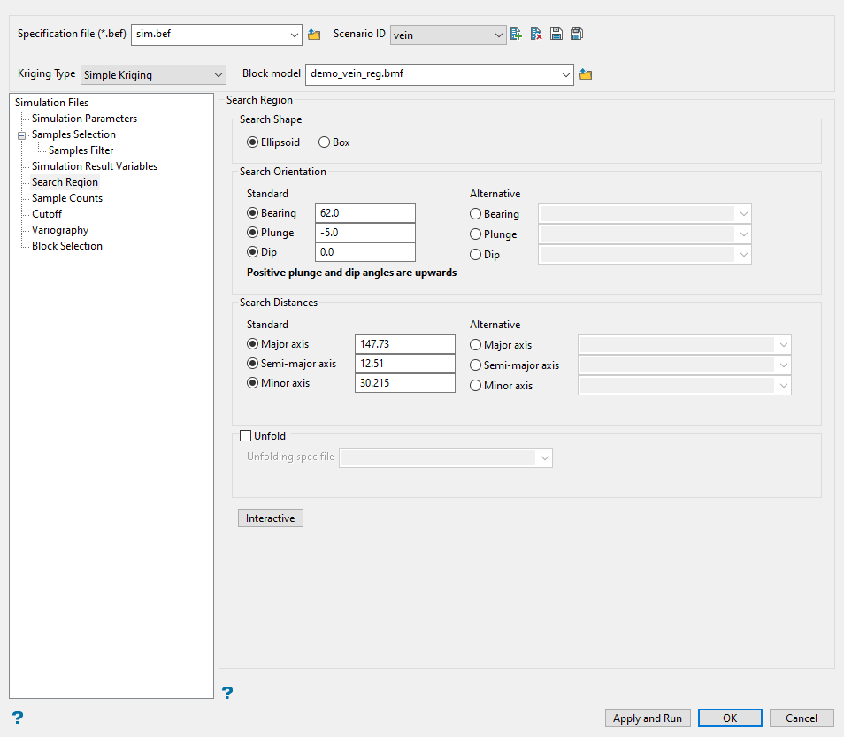
Use this pane to define the search distances and search orientation.

Follow these steps:

Select the shape of your search region.

Use search ellipsoid - Select this option to limit the search distance to an ellipsoid.

Use search box - Select this option to limit the search distance to a box instead of an ellipsoid.

Note: The volume of a box with sides 2a, 2b and 2c is about twice the volume of an ellipsoid with radii a, b and c. Therefore, when using the box search you collect about twice as many sample points. This causes an estimation using a box search to take from two to eight times as much time as an estimation with a search ellipsoid.
Enter the angles for the Bearing, Plunge, and Dip.

Note: You can enter the angles directly or select block model variables that contain the angles by choosing the Alternative options.

Search Orientation

The Bearing, Plunge and Dip values are angles, in degrees, that specify the orientation of the search ellipsoid and orientation of variogram structures. Care must be taken with these parameters as there are several common misunderstandings about the meaning of these parameters.

To understand these parameters, imagine an ore body with a primary axis. To find the bearing of the ore body, project the ore body axis straight up onto the surface plane and call this line the bearing line. The bearing is the angle clockwise from north to the bearing line.

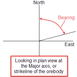
Figure 1: Bearing

Plunge is the angle between the horizontal plane and the ore body axis. Note that the plunge should be negative for a downward pointing ore body.

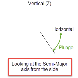
Figure 2: Plunge

To find the dip of an ore body, imagine the ore body is located in a plane. First rotate around the Z axis by the bearing so that the ore body is pointing north. Then rotate around the east-west axis by the plunge so that the ore body is level with the ground. At this point the ore body is parallel to the north-south axis. The dip is the angle of rotation to bring the plane into the horizontal plane. Looking north, if the plane must be rotated clockwise around the north-south axis, then the dip is positive (other software packages may use the opposite convention).

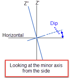
Figure 3: Dip

Note: The terms bearing, plunge and dip have been used by various authors with various meanings. In this panel, as well as kriging and variography, they do not refer to true geological bearing, plunge and dip. The terms X', Y' and Z' axis are used to denote the rotated axes as opposed to X, Y and Z which denote the axes in their default orientation.
Enter the dimensions of the search region.

Search Distances

The search box has sides with length twice the numbers given. The major axis radius is the search distance along the axis of the ore body. The semi-major radius is the search distance in the ore body plane perpendicular to the ore body axis. The minor axis radius is the search distance perpendicular to the ore body plane.

Note: Use the Display Ellipsoid option to verify that you are using the proper orientation angles. Display the search ellipsoids over your sample data to verify the correct orientation of the ellipsoid.

The search radii are true radii. If you set your major search radius to '100', then the ellipsoid has a total length of 200. The following diagram shows the relationship between the axes with the ellipse in the default orientation (bearing 90°, plunge and dip 0.00°).

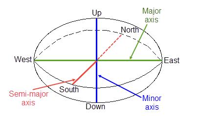
Figure 4: Relationship between Radii
Select Unfold to use a tetrahedral model. This is applicable only for folded or faulted block models for which a tetrahedral model has been created.
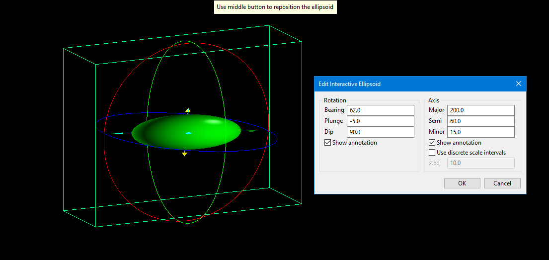
Click the Interactive button to adjust the search distances and orientation visually.
1. Set the origin by selecting a location on the screen. This point is an arbitrary point used to define the starting location for measuring the distance and orientation.
2. Set the parameters for rotation by adjusting the Bearing, Plunge, and Dip. Set the parameters for the distances by adjusting the Major, Semi, and Minor settings. You can do this by entering the numbers manually, or by clicking and dragging the arrows and rings on the screen.
3. Select Show annotations to toggle the display for showing the arrows.
4. Select Use discrete scale intervals to limit increasing or decreasing the distances by the Step size you enter.
5. Click OK to return to the main panel.

Sample Counts

Use this pane to define the number of samples used for each block in the simulation.

Follow these steps:

Enter the minimum number of samples that have to be found to generate an estimate in the field Minimum number of samples per estimate. Blocks with less than this number of samples within the search ellipsoid or box are assigned the default grade value.
Enter the maximum number of samples to be used in any grade estimation in the field Maximum number of samples per estimate.

Example: The estimation program may find 30 samples near a block centre. If you had specified a maximum of 10 samples, then only the 10 samples closest to the block centre would be used. The distance to the block centre is calculated by an anisotropic distance based on the search radii. Up to 999 samples per estimate are allowed.
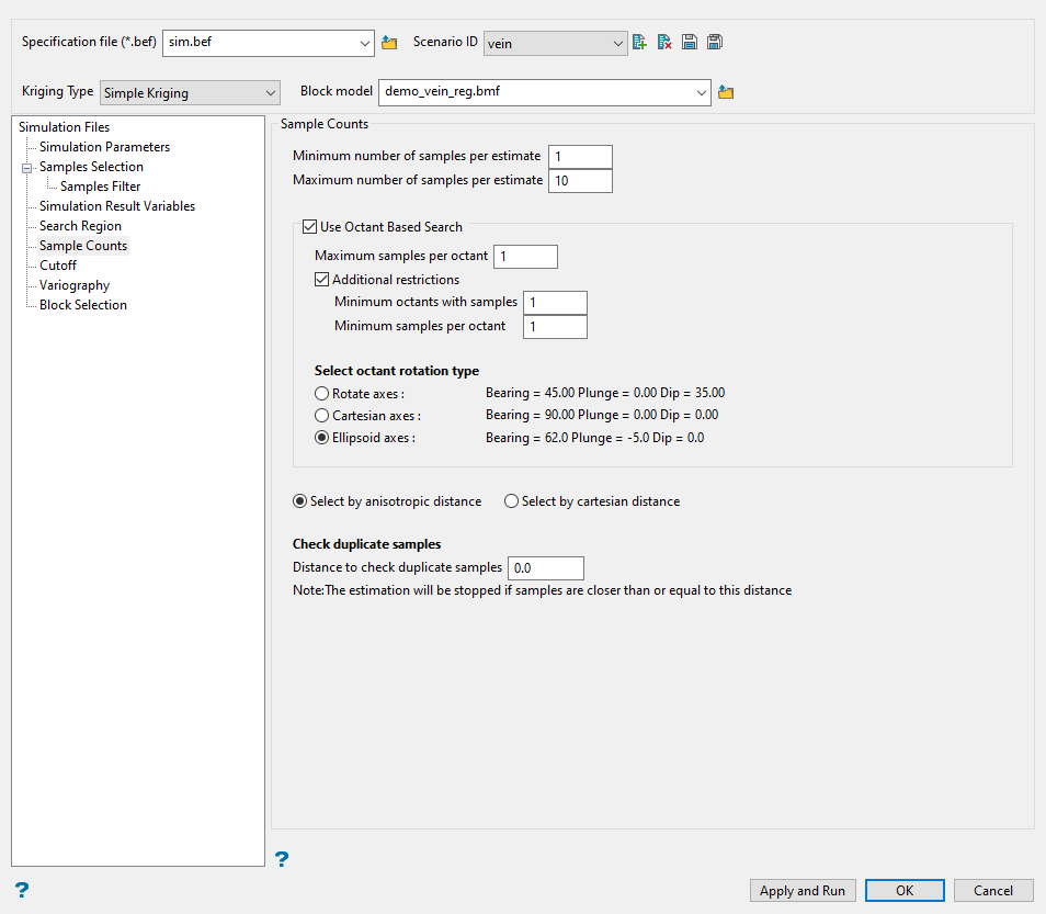
Select Use an octant based search if you want to place a limit on the number of samples that can come from a given octant. The space around a block centre is divided into eight octants by three orthogonal planes. You have a choice of plane orientations, Rotate axes, Cartesian and Ellipsoid axes.
Enter the maximum number of samples from each octant to be used in the field Maximum samples per octant. Samples closest to the block centre are used first.

Note: The maximum number of samples per estimate always applies, regardless of the maximum samples per octant value.

Select Additional restrictions if you want to apply additional restrictions to the number of samples for octants. These restrictions comprise of minimum octants with samples and minimum samples per octant.

The Minimum octants with samples enables you to specify the number of octants that must contain samples for an estimate to be generated.

The Minimum samples per octant enables you to specify the number of samples per octant that needs to be found to generate an estimate.

These two restrictions work together. An octant is considered filled if it contains at least the minimum number of samples per octant. The minimum number of octants with samples requires that at least that number of octants be filled.

Example

If you set the minimum number of samples per octant to 2, the minimum number of octants to 3 and have the following number of samples per octant, there are two filled octants. As this is less than the minimum number of octants with samples, the default value is assigned to this block.

Octant Number	Number of samples per octant	Filled / Not Filled
0	1	Not filled
1	3	Filled
2	2	Filled
3	1	Not filled
4	1	Not filled
5	1	Not filled
6	1	Not filled
7	0	Not filled

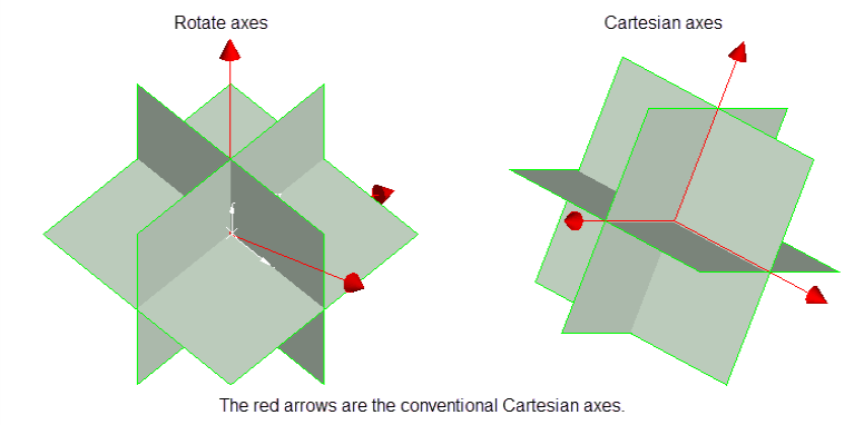
Select octant rotation type. This option is only available if you are using an octant based search.
- Rotate axes - This consists of three planes perpendicular to axes that have been rotated 45° about the Z axis and 35° about the X' (X axis after rotation about the Z axis). It produces a set of planes where the first has a bearing of 135°, the second has a bearing of 45° and is at angle of -55° to the horizontal and the third also has a bearing of 45°, but is at an angle of 35° to the horizontal, see the diagram below.
- Cartesian axes - This consists of three planes perpendicular to the conventional Cartesian axes X, Y and Z (or East, North and elevation) axes.
- Ellipsoid axes - This consists of three planes that are perpendicular to the major, semi-major and minor axes of the search ellipsoid.
Note: An octant search is a declustering tool used to reduce imbalance problems associated with samples lying in different directions. If there are more samples in one direction than another, then this option limits the bias.

The samples are sorted by distance (either Anisotropic or Cartesian) prior to the samples being limited. This ensures that the closest samples are kept.
Choose either Select by anisotropic distance or Select by Cartesian distance.
- Select by anisotropic distance - Select this option to use the anisotropic distance defined by the ellipsoid axes to determine the samples that are closest to the block centroid.
- Select by Cartesian distance - Select this option to use the Cartesian distance to determine the samples that are closest to the block centroid.
Enter the Distance to use to check duplicate samples in the field provided. Samples less than or equal to the specified distance value are considered to be duplicates, resulting in the entire grade estimation process being stopped. You can disable this feature by specifying a distance value of '-1'.

Cutoff

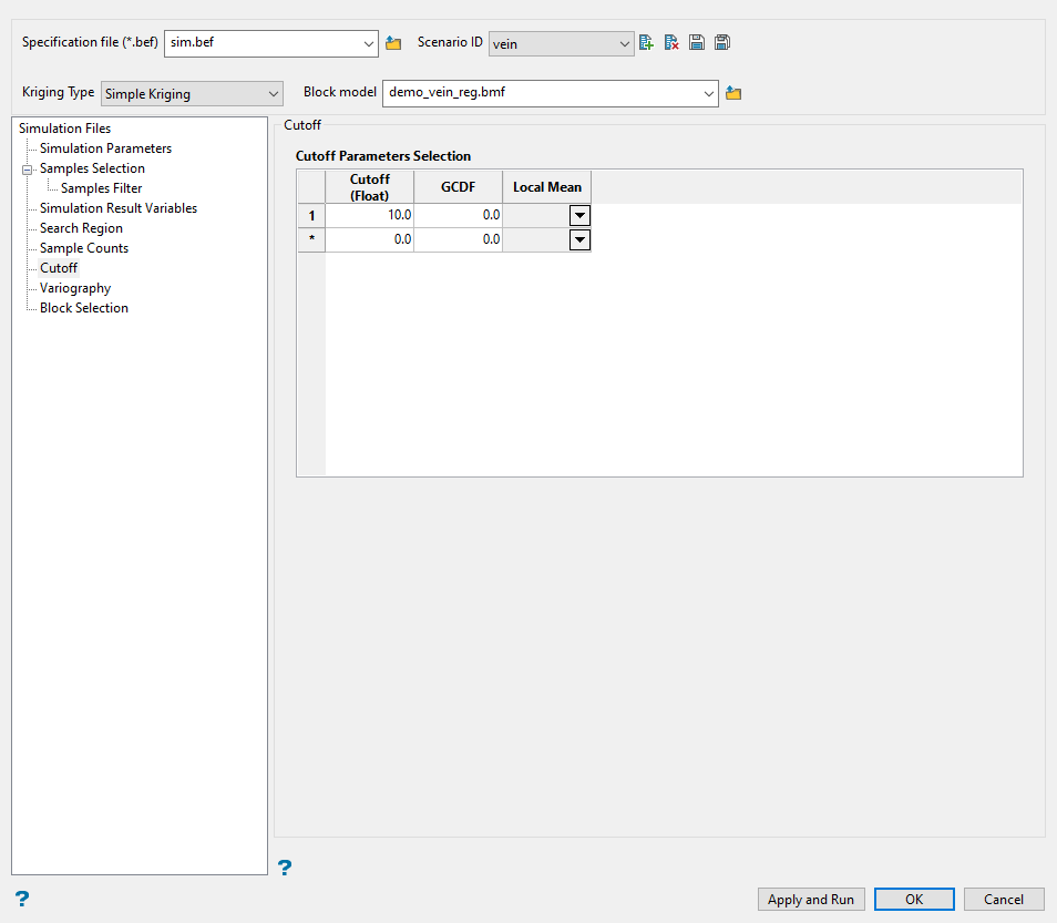
Use this pane to set the cutoff thresholds and select the variable used to hold local mean values.

Follow these steps:

Enter the grade Cutoff threhold. The cutoffs should be entered from lowest cutoff to highest cutoff. A sample value equal to the cutoff is considered to be in the interval above the cutoff.
Enter the GCDF (Global Cumulative Distribution Function) values of a distribution function at each cut-off level. The values should be from 1.0 to 0.0 and decreasing. When no sample data is available for a block, the simulated value is chosen from this distribution. It is often desirable that the GCDF not produce high grade values.

You can assure this by having the GCDF value approach 0 quickly. It is reasonable that the GCDF be 0 for all high cut-offs. If you want all default values to be less than the lowest cut-off, set all the GCDF values to 0.
Select the variable that holds the local mean value.

Note: This option is only available if you are using the kriging method Simple kriging with local mean.
Click the Variography tab to continue.

Variography

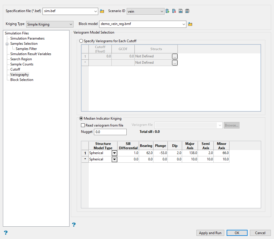
Use this pane to define either a variogram for each cut-off or specify the variogram that will be used for all cut-offs.

Follow these steps:

Select Specify variograms for each cutoff or Median Indicator Kriging.
- Specify variograms for each cutoff - Use a variogram for each cut-off. If you select this option the table will be populated using information from the Cutoff pane.
  1. Click the icon in the Structs column to display the panel from which you will select your variograms for each cutoff.
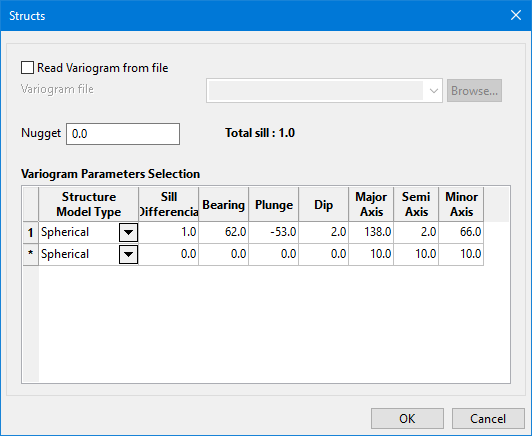
  2. Select Read variogram from a file to use an existing variogram model. Use the drop-down list to select the model. Variogram models are stored in (.vrg) files.
  3. Enter the nugget.
  4. Select the type of model from the drop-down list labelled Structure Model Type.
    
    The variogram model type can be one of the following:
    
    Spherical
    
    This type is the most commonly used for ore deposits. They exhibit linear behaviour at and near the origin then rise rapidly and gradually curve off.
    
    Exponential
    
    This type is associated with an infinite range of influence.
    
    The sill is reached at the specified range parameter. In release 3.2 and earlier, users were required to enter a range parameter of one-third the practical sill range. To use this model, enter the practical distance of the sill as a range parameter. For backward compatibility, see the Exponential Model 3.
    
    Gaussian
    
    This type exhibits parabolic behaviour at the origin and, like the spherical model, rises rapidly. The Gaussian type reaches its sill smoothly, which is different from the spherical model, which reaches the sill with a definite break. The Gaussian model is rarely used in mineral deposits of any kind. It is used most often for values that exhibit high continuity.
    
    In release 3.2 and earlier, users were required to enter a sill range of 3 times the actual sill range. To use this model, enter the effective range of the sill. For backward compatibility, see the Gaussian model 3.
    
    Linear
    
    This type is a straight line with a slope angle defining the degree of continuity.
    
    De-Wijsian
    
    This type is a representation of a linear semi-variogram versus its logarithmic distance.
    
    Power
    
    This type is computed as M - d**p where M = the maximum correlation defined as 1000.0, d = distance from the origin, p = model power. For this model type only the power p is the major axis radius. Adjust the size of the ellipsoid so that the major axis is the desired power. The size of the ellipsoid for this model does not change the calculation of the variogram.
    
    Exponential Model 3
    
    This is an un-normalised exponential model for compatibility with release 3.2 and earlier. This variogram will have the practical sill at three times the distance entered as range parameter.
    
    Periodic
    
    This is a sine wave with one complete period over the effective range. This model is not commonly used because it can cause samples at greater distances to have higher correlation.
    
    Gaussian Model 3
    
    This is an un-normalised Gaussian model for compatibility with release 3.2 and earlier. The input radius must be the effective radius multiplied by 3.
    
    Dampened Hole Effect
    
    Dampening is achieved by multiplying the covariance function by an exponential covariance, that acts as a dampening function.
  5. Enter the Sill Differential. This represents the difference between the value of the variogram where it levels off and the nugget. For example, if you have a total sill of 1.0, and a nugget of 0.15, you want your sill differential to be 0.85 = (1.0 - 0.15).
    
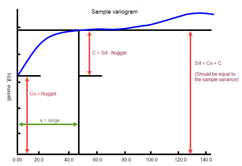
    In the diagram, C₀ is the nugget, and C is the sill differential.
  6. Enter the Bearing (Rotation about the Z axis), Plunge (rotation about the Y axis), and Dip (rotation about the X axis) of the variogram.
  7. Enter the radii of the Major, Semi, and Minor axes of the variogram.
- Median Indicator Kriging - Use one variogram that will be used for all cut-offs. You can use an existing variogram file or enter the parameters directly into the table, as just described above.

Block Selection

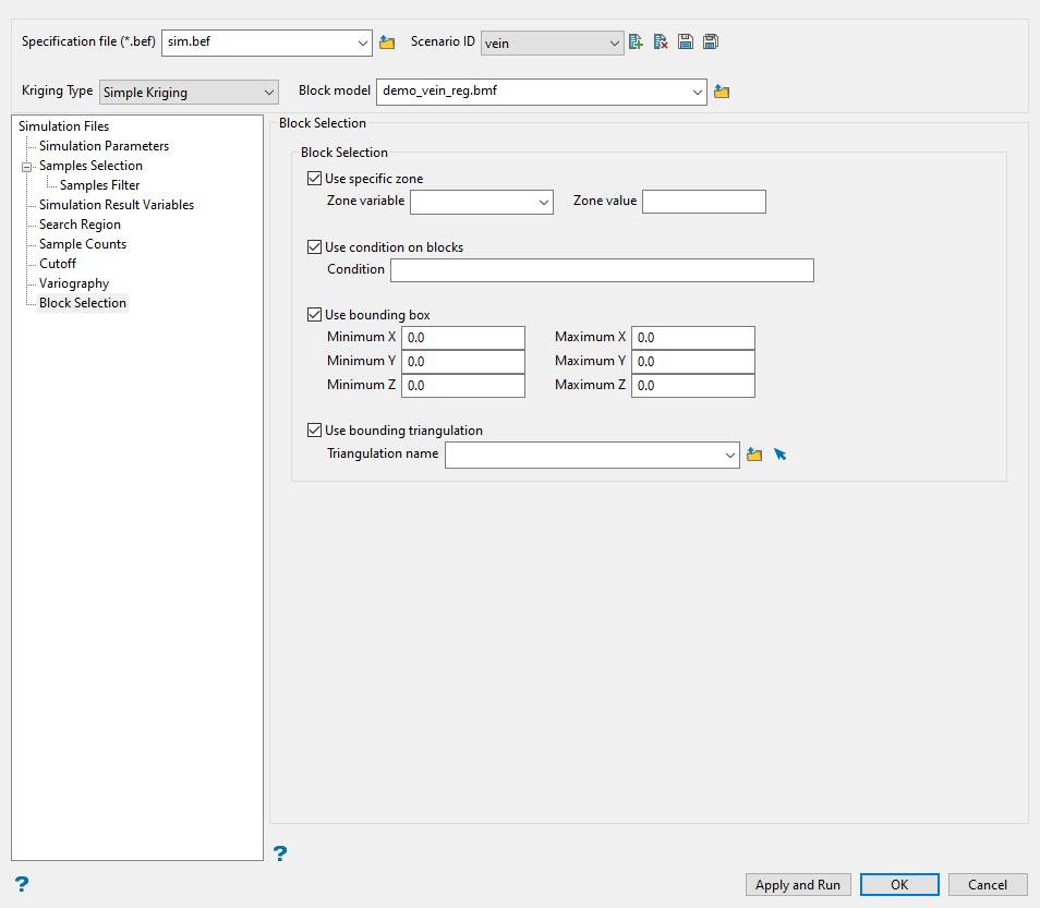
Use this pane to limit the blocks that will be used. All of the selections on this pane are optional.

Options available:

Click Apply and Run to begin the simulation. This will save your settings in to the specification file and start the simulation run.

Click OK to save your settings to the specification file without running the simulation.

Click Cancel to close the panel without saving any settings.