Geostatistical Modelling
Structural Analysis - Variography
Neighbouring samples from a common geological environment are expected, on average, to exhibit more similarity in their assay values and have smaller differences, than samples taken from further apart. The greater the distance between the samples, the greater the difference is expected to be.
It therefore seems logical to find a way to examine the magnitude of the differences of samples at various distances, which would also characterise the degree of similarity or dissimilarity of the samples. This is generally done in a geologically defined homogenous zone . A semi-variogram can be used to define the spatial correlation between the values of a variable in the field of interest.
A natural manner in which one would compare neighbouring assays would be to plot the difference between pairs of samples. However, the sign of the difference is not of concern, and dealing with only a single pair of samples at a time is of very little value. Thus, the absolute value of the average differences of all the pairs which are h distance apart is considered. To further pronounce the magnitude differences and to avoid mathematical difficulties that may arise from using absolute values, the mean squared differences are computed and plotted as a variogram.
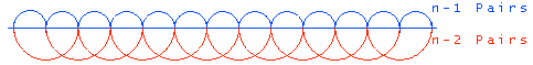
The semi-variogram is therefore defined as half the mean squared difference of pairs of values at some distance h apart. To illustrate the method of calculation, consider a set of samples taken at regular intervals of 1 metre along a straight line (Fig. 4). To generate a semi-variogram it would be required to calculate the half mean squared differences of all the samples 1 metre apart (that is, n-1 pairs). Then repeat the process for samples which are 2 metres apart (n-2 pairs) and so on.
Figure 4 - Process of Semi-Variogram Generation