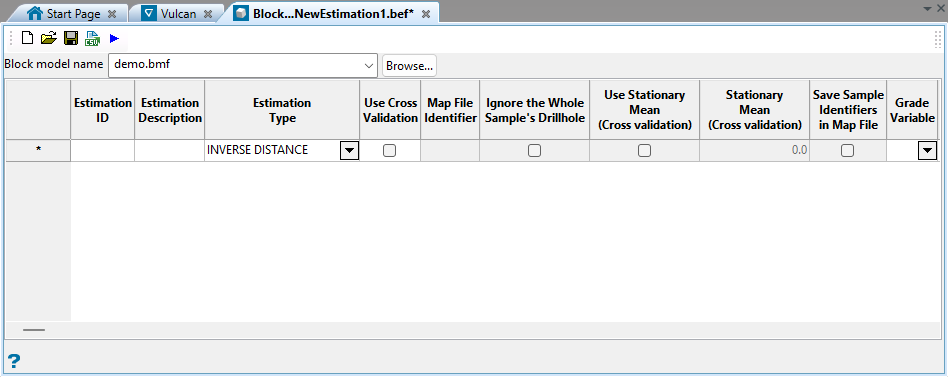
New Estimation File
Use this option to create a new block estimation file (.bef). The format of the file name is (<proj><name>.bef).
You can create a new block estimation file in one of three ways:
- Select Block > Grade Estimation > New Estimation File.
- Right-click on the Grade Estimation folder in the Specifications folder (of the Vulcan Explorer) and select New Block Estimation File from the displayed context menu.
- Select the
 New option from the Block Model Utility.
We recommend that you create your first estimation file by using the appropriate option in the Block > Grade Estimation submenu. Once created, you can use the Block Model Utility to update the estimation parameters.
Important: Multi-thread estimation requires clean data in order to work correctly. Duplicated samples are not allowed.
Instructions
On the Block menu, point to Grade Estimation, then click New Estimation File to display the Block Model Utility window.
Listed in alphabetical order.
Select this check box to apply additional restrictions to the number of samples for octants. These restrictions comprise of minimum octants with samples and minimum samples per octant.
The minimum octants with samples enables you to specify the number of octants that must contain samples for an estimate to be generated. The minimum samples per octant enables you to specify the number of samples per octant that needs to be found to generate an estimate. These two restrictions work together. An octant is considered "filled" if it contains at least the minimum number of samples per octant. The minimum number of octants with samples requires that at least that number of octants be filled.
If you set the minimum number of samples per octant to 2, the minimum number of octants to 3 and have the following number of samples per octant, there are two filled octants. As this is less than the minimum number of octants with samples, the default value is assigned to this block.
| Octant Number | Number of samples per octant | Filled / Not Filled |
|---|---|---|
| 0 | 1 | Not filled |
| 1 | 3 | Filled |
| 2 | 2 | Filled |
| 3 | 1 | Not filled |
| 4 | 1 | Not filled |
| 5 | 1 | Not filled |
| 6 | 1 | Not filled |
| 7 | 0 | Not filled |
This option is only available when using the inverse distance method. When you define the inverse distance method you define radii that control the inverse distance weighting. If you normalise your inverse distance weights to the search ellipsoid radii, these distances are the same as the distances derived from the search ellipsoid.
Either unweighted or weighted distances can be stored. If unweighted, then all samples are given the same weight. If weighted, the weights used for grade estimation are applied.
Suppose we are estimating a block and have two samples. Sample 1 is at a distance of 10 and Sample 2 is at a distance of 100. Suppose, also that Sample 1 has a weight of 0.95, and Sample 2 has a weight of 0.05. The unweighted distance is (10+100)÷2 or 55. The weighted distance is (0.95×10 + 0.05×100) or 14.5.
If your search ellipsoid is spherical (major, semi-major and minor radii are the same) this anisotropic distance is the same as the Cartesian distance. Suppose, however, that your search ellipsoid has radii of 100, 50 and 10. This means that points in the direction of the semi-major axis have their distances expanded by a factor of 2 = (100/50) and points in the minor direction have their distances expanded by a factor of 10 = (100/10). In general, anisotropic distances are computed as:
where:
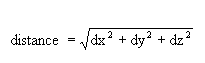
dx, dy, and dz are the distances in the major
semi-major and minor directions
anisox, anisoy, and anisoz are the anisotropic weighting factors.
The anisotropic weighting factors cause any samples that lie on the surface of the search ellipsoid to have the same anisotropic distance, namely, the major axis radius.
Enter the anisotropic radii. These values are used to calculate the anisotropic weightings applied to each of these axes.
These weightings are a ratio of the lengths of the major, semi-major and minor radii. Thus the major (X) axis weighting is 1 (one), the semi-major (Y) axis weighting is the length of the major radius divided by the length of the semi-major radius, and the minor (Z) axis weighting is the length of the major axis radius divided by the length of the minor axis radius. Please note that it is possible to use equivalent ratios. That is 1:0.5:0.2 is the same as 10:5:2. The weightings are the inverse of the radii ratios.
If the ratio is 1:0.5:0.2, then the weightings are 1, 2 and 5. The Distances to Samples panel (in Grade Estimation) and the New Estimation File option uses these weights for the Anisotropic distance derived from the anisotropic weights option.
Select this option to apply the base logarithm function to all sample values.
All original sample values must be positive for the logarithm t o be defined. The specified logarithm constant is added to the calculated logarithm.
Specify the field containing the samples to be estimated.
Select this check box to estimate sub-blocks as if they were the parent block. This means that instead of using the block extent of the sub-block, the estimation procedure uses the extent of the parent block.
Suppose we have a primary scheme of block size of (50, 50, 50) and we are estimating a block whose extent ranges from (60, 30, 50) to (70, 40, 70). This block has sides of length 10, 10, and 20. The parent block that contains the sub-block ranges from (50, 0, 50) to (100, 50, 100). The parent block has sides of 50, 50 and 50 and has centre at (75, 25, 75). This block is estimated as if its centre were at (75,25,75) and as if its sides were 50, 50 and 50.
It is also possible to enter the parent block size. You will need to enable the Choose parent block size (Grade Estimation) or Enter Parent Block size (Block Model Utility ) check box, and then enter the lengths of the block.
Up to 3 decimal places may be entered in the Parent Block XYZ fields.
If any type of block selection is used, then not all sub-blocks in a parent block have the same value. A sub-block is only estimated if it is selected by the block selection procedure. For example, suppose you have two zones, 'ORE' and 'ROCK'. When you estimate blocks in the 'ORE' zone, only blocks actually in the ore zone are updated. Blocks in the 'ROCK' zone are not updated, even if they are in the same parent block. If you want all blocks in a parent block to have the same grade value, then you need to run grade estimation on all the sub-blocks. The easiest way to do this is to run grade estimation without any block selection conditions.
If this check box is not selected, then the true block extents and sizes are used instead.
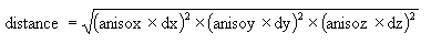
The Bearing, Plunge and Dip values are angles, in degrees, that specify the orientation of the search ellipsoid and orientation of variogram structures. Care must be taken with these parameters as there are several common misunderstandings about the meaning of these parameters.
To understand these parameters, imagine an ore body with a primary axis. To find the bearing of the ore body, project the ore body axis straight up onto the surface plane and call this line the bearing line. The bearing is the angle clockwise from north to the bearing line.
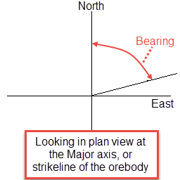
Figure 1: Bearing
Plunge is the angle between the horizontal plane and the ore body axis. Note that the plunge should be negative for a downward pointing ore body.
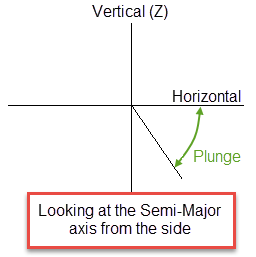
Figure 2: Plunge
To find the dip of an ore body, imagine the ore body is located in a plane. First rotate around the Z axis by the bearing so that the ore body is pointing north. Then rotate around the east-west axis by the plunge so that the ore body is level with the ground. At this point the ore body is parallel to the north-south axis. The dip is the angle of rotation to bring the plane into the horizontal plane. Looking north, if the plane must be rotated clockwise around the north-south axis, then the dip is positive (other software packages may use the opposite convention).

Figure 3: Dip
The terms bearing, plunge and dip have been used by various authors with various meanings. In this panel, as well as kriging and variography, they do not refer to true geological bearing, plunge and dip. The terms X', Y' and Z' axis are used to denote the rotated axes as opposed to X, Y and Z which denote the axes in their default orientation.
Enter the bearing, plunge and dip of the restricted search region.
Sample selection must be configured so that the samples that belong to the estimation domains needed here are selected. If the sample selection criteria does not allow for samples in soft boundaries domains to be selected, then no samples will be applied the definitions specified here.
Enter, or select from the drop-down list, the name of the block model on which the estimation will be performed.
The block model name is stored in the .bef file, and is used if the block estimation is performed in the Workbench. The resulting .bef file can also be used externally in a shell window. However, in the latter case the estimation file does not recognise the stored block model name.
The remainder of the panel consists of a series of columns that are described in detail below. Any cells that are coloured pink are mandatory.
The distance from the block centre is computed using the Pythagorean formula:
If no weighting is used, then each sample is given an equal weight. If weighting is used, then the weights used in grade estimation are applied. When performing indicator kriging, the weights of the first cutoff are used.
Select the character field to which you want to limit the samples.
Select this check box to apply cut-offs to the grades used in the estimation. Specify a lower grade cut value (grades lower than this value are set to this value) and an upper grade cut value (grades above this value are set to this value).
Select Database or Mapfile or ODBC Link to indicate the database type.
This value refers to the number that will be stored as an average distance if there aren't enough samples available to make an estimate.
Enter the default value. This value, which can contain up to 3 decimal places, is stored in the variable if it is less than the minimum number of valid samples is available.
Select the ![]() Save option to save the new estimation settings. This option will also save the current view settings for the estimation file.
Save option to save the new estimation settings. This option will also save the current view settings for the estimation file.
If you have chosen to remove the Map File Identifier column from view, that is, you have hidden the column through the Select Columns option, then this column will remain hidden until its visibility setting is restored and the changes to the estimation file are saved.
Click  Export parameters to a CSV file to save the block estimation file (
.bef) parameters to a CSV file. Enter a File name in the Save panel that is displayed and click Save to save the file to the current working directory, or navigate to another location to save the CSV file to a different folder.
The exported CSV file has two header rows, the first containing the key for each parameter (a coded name with no spaces) and the second containing the full parameter names (written out titles).
To run the block estimation, select the  Run Estimation option in the Block Model Utility. You can also add these new parameters to an existing block estimation run file (
.ber) in the Open Estimation Run File option, or add them to a new file through using the New Estimation Run File option.
Once this has been done, select the Execute Estimation Run File option to execute the run file and the nominated block estimation parameters.
Enter the value to be stored in the estimation variable for blocks that are not estimated. The value does not have to be the same as the default specified when creating the block model.
The variance is obtained by discretising the block and calculating the average variogram value for all possible pairs. The X, Y, Z discretisation parameters control the number of pairs to consider. In practice, a 5 x 5 x 5 discretisation is appropriate to obtain a robust estimate of the average variogram. Too many points may lead to numerical precision problems. A large number of grid points can cause Vulcan to run slowly. A 4 × 4 × 4 grid is usually sufficient. In no case should there be more than 10,000 grid points.
Enter the distance to use to check duplicate samples. Samples less than or equal to the specified distance value are considered to be duplicates, resulting in the entire grade estimation process being stopped. You can disable this feature by specifying a distance value of '-1'.
There are three different kinds of distances that can be stored (standard Cartesian, and anisotropic distance derived from the search ellipsoid, and anisotropic distance which is derived from anisotropic weights ). In addition there are weighted and unweighted interpretations of each of these, for a total of six different kinds of distance. Any, all, or none of the different distance measures can be stored by putting a block model variable name in the appropriate panel item. If you do not want to store a value, then leave the panel item blank.
Specify the database field name that contains the drillhole name. This field will only be displayed when using the Store Num Holes option.
Select this option to enable the fields allowing you to enter the parent block sizes in the X, Y, and Z direction.
Enter the estimation ID (a maximum size of 6 alphanumeric characters).
Select the type of estimation to use. Only authorised estimation types displays in the drop-down list, that is, if a geomodeller licence configuration is being used then only 'INVERSE' will be shown.
Select this check box to ignore sample values at or above the specified threshold and outside the specified ellipsoid.
Select this check box to apply the same weights to several sample variables. For example, if you have several different metals that follow the same variography, you may want to use the same weights for each of your metal variables.
Enter the field selection criteria, remember do not use spaces in the conditions.
Enter, or select from the drop-down list, the name of the block model variable in which to store the estimate of the grade.
Note: The variable must be a float or double data type. Refer to the Block > Transfer > Regularise Model option for more information on data types.
Specify the database field that contains the high yield limit. It is usually the same as the input grade field. However, other fields can be used to achieve special sample limits.
Note: You can specify a flag field here, where 0 represents an ordinary sample and 1 represents a special sample. A threshold of 0.5 would then limit the flagged samples to a smaller radius.
Enter the threshold you want to use as a limit for high-yield samples. Only samples that are less than the threshold will be used.
When setting a high yield limit, the value caps the sample outside of your specified distance & angle parameters. The high yield exclusion ellipsoid specified through this section of the Estimation Editor interface has its own major, semi-major and minor axes that have the same orientation as the ellipsoid defined through the Search Region section. When selecting the samples for the grade estimation, any samples within the high yield exclusion ellipse can be chosen whether they are greater than or less than the threshold. However, between the smaller high yield exclusion ellipse and the normal Search Region ellipse, only samples that are less than the threshold can be chosen. This is commonly used to avoid estimation from high gold nugget values to distant blocks.
Suppose we have several high-value samples that we would still like to use in our estimation and they outside of our high value spatial limits. We set the Threshold value to a lower value. Then, we set our XYZ distance and rotation. Within that bubble, the high-value samples will be used without capping. Outside of that bubble, the value will be reduced to the lower value.
If you want to use a customised orientation for the search ellipsoid, enable the checkbox labelled High yield limit use angles, then enter the bearing, dip, and plunge into the spaces provided.
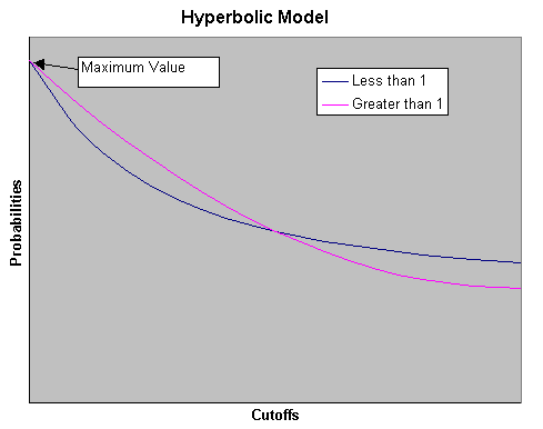
This option gives a distribution with no maximum. If the power is greater than 1, then the distribution contains more values closer to the highest cut-off and less higher values. Whereas if the power is less than 1, then the distribution contains less values closer to the highest cut-off, but more higher values. The hyperbolic model right tail option always allows for the possibility of arbitrarily large simulated values.
Select this check box to ignore specific character values. Ignoring specific character strings may be useful to eliminate certain strings, for example, waste, from being included in the grade estimation.
Select this check box to ignore specific numeric values. This feature is useful for eliminating certain negative values from being included in your grade estimation.
Select this check box to ignore the currently used sample and all the drillhole data associated with it. Do not select this check box if you only want to ignore the sample that is currently in use.
Specify the numeric values that you want to ignore. To do this, click on the button to the right of the cell. A new column displays. Enter each value on a new line.
Select the variogram model type to be used from the drop-down list. The variogram model type can be one of the following:
The variogram model type can be one of the following:
Spherical
This type is the most commonly used for ore deposits. They exhibit linear behaviour at and near the origin then rise rapidly and gradually curve off.
Exponential
This type is associated with an infinite range of influence.
The sill is reached at the specified range parameter. In release 3.2 and earlier, you were required to enter a range parameter of one-third the practical sill range. To use this model, enter the practical distance of the sill as a range parameter. For backward compatibility, see the Exponential Model 3.
Gaussian
This type exhibits parabolic behaviour at the origin and, like the spherical model, rises rapidly. The Gaussian type reaches its sill smoothly, which is different from the spherical model, which reaches the sill with a definite break. The Gaussian model is rarely used in mineral deposits of any kind. It is used most often for values that exhibit high continuity.
In release 3.2 and earlier, you were required to enter a sill range of 3 times the actual sill range. To use this model, enter the effective range of the sill. For backward compatibility, see the Gaussian model 3.
Linear
This type is a straight line with a slope angle defining the degree of continuity.
De-Wijsian
This type is a representation of a linear semi-variogram versus its logarithmic distance.
Power
This type is computed as M - d**p where M = the maximum correlation defined as 1000.0, d = distance from the origin, p = model power. For this model type only the power p is the major axis radius. Adjust the size of the ellipsoid so that the major axis is the desired power. The size of the ellipsoid for this model does not change the calculation of the variogram.
Exponential Model 3
This is an un-normalised exponential model for compatibility with release 3.2 and earlier. This variogram will have the practical sill at three times the distance entered as range parameter.
Periodic
This is a sine wave with one complete period over the effective range. This model is not commonly used because it can cause samples at greater distances to have higher correlation.
Gaussian Model 3
This is an un-normalised Gaussian model for compatibility with release 3.2 and earlier. The input radius must be the effective radius multiplied by 3.
Dampened Hole Effect
Dampening is achieved by multiplying the covariance function by an exponential covariance, that acts as a dampening function.
Refer to the Variogram Model Types section for a more detailed explanation of the mathematics related to variograms and diagrams of the variogram model types.
Enter the sill differential. This represents the difference between the value of the variogram where it levels off and the nugget. For example, if you have a total sill of 1.0, and a nugget of 0.15, you want your sill differential to be 0.85 = (1.0 - 0.15).
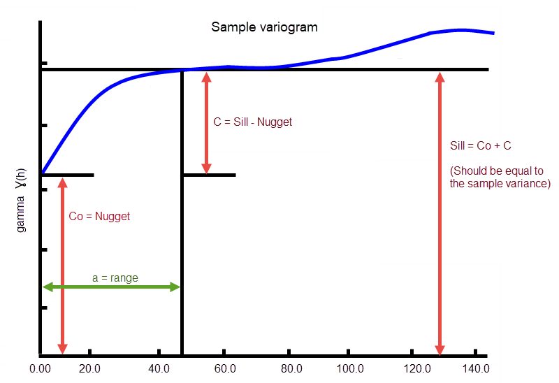
Figure 4: Sample Variogram
In the diagram, C0 is the nugget, and C is the sill differential.
Enter the grade cut-off level. The cutoffs should be entered from lowest cutoff to highest cutoff. A sample value equal to the cutoff is considered to be in the interval above the cutoff.
Enter the value to store for the indicator and variance when the block is not estimated.
Enter the value of the nugget (C0 ).
Using a nugget value of 0 (zero) will not weight everything equally; rather, using a nugget value without setting up additional variography models will cause equal weighting. A nugget value of 0 is valid; however, not recommended from a geostatistical standpoint. A nugget represents the variability at 0 distance and is typically between 0.05 and 0.2.
Select the block model variable to store the indicator variable. In version 3.2 and earlier, it was necessary to store every indicator variable in the block model and run a script afterward to produce an estimated grade. Later releases contain a post-processing option to produce a total grade based on defined interval means, or to sample the distribution and store specific values derived from the distribution. It is not necessary to store all the indicator variables.
Select the variable in which to store the kriging variance from the variogram model for this cutoff.
Enter the required number of variogram structures.
If you have more than variogram structure, then the following columns are displayed for each structure. If the columns are not displayed, then use the Select Columns command to update the column visibility.
Enter the number of cutoffs required.
If you have more than one cut off, then the following columns are displayed for each cut off. If the columns are not displayed, then use the Select Columns command to update the column visibility.
Enter the sample variable from the mapfile or Isis composites database.
Select this check box to limit the number of samples per drill hole that can be used in the estimation. Enter the maximum number of samples per drill hole and specify the name of the database field containing the drill hole name. The default is DHID.
The estimation uses the samples closest to the centre of the block.
Enter, or select from the drop-down list, the fields containing the X, Y and Z coordinates. Field names can either be entered manually or selected from the drop-down list. In ordinary or indicator kriging, if two samples have the same coordinate, then they are treated as if there were a very small distance between them. This means that the kriging process does not produce a singular matrix when sample points are coincident. Also, if a sample point is coincident with a block centre, then it is not taken as the block value.
Enter the radii for the high yield exclusion ellipsoid.
Enter the radii for the restricted search ellipsoid.
Specify the mapfile identifier of the ASCII mapfile that contains the desired sample data.
Enter the maximum number of previously estimated blocks to use. As stochastic simulation proceeds, it collects samples from previously estimated blocks and from sample data.
Enter the maximum number of samples to be used in any grade estimation. For example, the estimation program may find 30 samples near a block centre. If you had specified a maximum of 10 samples, then only the 10 samples closest to the block centre are used. The distance to the block centre is calculated by an anisotropic distance based on the search radii. Up to 999 samples per estimate are allowed.
Enter the maximum number of samples from each octant to be used in the estimation. Samples closest to the block centre are used first.
The maximum number of samples per estimate always applies, regardless of the maximum samples per octant value.
Enter the highest value of the specified numeric range.
Enter the minimum number of valid samples that are allowed for an estimate. If at least this many valid samples values are available, an estimate of this variable is made. This minimum may be less than the minimum number of samples.
Suppose you specified a minimum of 5 samples per estimate and a minimum number of valid samples for a variable as 2. Then suppose that a block had 5 samples selected. This means that up to 3 of the samples could be missing and an estimation of that variable is still made. However, if 4 of the 5 samples were missing, then the estimate would not be made and the default value would be stored for that variable.
Enter the minimum value that is considered valid for this variable. Sample values below this value are considered missing. If your grade values are all positive and you use -1 or -9 as a missing data flag, putting 0 for this value is a good idea. The specified value can contain up to 3 decimal places.
Enter the smallest possible value in the distribution. This value should be less than the smallest cut-off.
Enter the minimum number of samples that have to be found to generate an estimate. Blocks with less than this number of samples within the search ellipsoid or box are assigned the default grade value.
Enter the lowest value of the specified numeric range.
Click Normalise to calculate the anisotropic weightings normalised to the search radii. The distances used here are those entered into the Standard Major, Semi-major, and Minor axis settings found on the Search Region pane. You may still edit the weightings.
If you are using an ODBC database, select the ODBC design to use from the drop-down list. This option is only enabled if you selected ODBC Link in the Database Type field.
Specify the variable in the block model to receive the weighted estimate. You must select one block model variable for every input variable you select.
Enter the size of the parent block in the X direction.
Enter the size of the parent block in the Y direction.
Enter the size of the parent block in the Y direction.
Select the variable holding the size of the parent block in the X direction.
Select the variable holding the size of the parent block in the X direction.
Select the variable holding the size of the parent block in the X direction.
Enter the power for the interpolation curves. This describes the shape of the curve between cut-off values. If it is less than 1, then the distribution is skewed towards the left. If it is greater than 1, then it is skewed towards the right between cut-offs. If it is equal to 1, then the distribution is flat between cut-offs.
This describes the shape of a curve from the Minimum data value to the lowest cut-off. If this value is less than 1, then the distribution is skewed towards the minimum data value. If it is greater than 1, then the distribution is skewed towards the lowest cut-off. If it is equal to 1, then the distribution is flat from the minimum data value to the lowest cut-off.
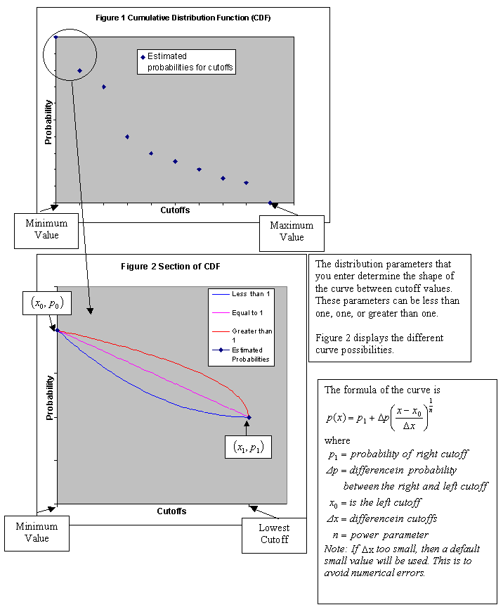
This option gives a distribution with a maximum data value. The maximum data value should be larger than the highest cut-off. The power for the right tail curve controls the shape of the distribution above the highest cut-off. If the power is less than 1, then the distribution is skewed towards the highest cut-off. If the power is greater than 1, then the distribution is skewed towards the maximum data value.
Enter the power to use on the inverse distance. A value of 2.0 means inverse distance squared while a value of 3.0 means inverse distance cubed, etc.
Enter the random number seed. The random numbers used by Vulcan are actually pseudo-random numbers that can be reproduced by starting with the same initial conditions. The random number seed controls which sequence of random numbers Vulcan uses. By using the same random number seed, previous results can be reproduced. Hence by using different random number seeds, different simulations are produced. Each stochastic simulation run only produces one possible set of values in the block model. It is desirable to run several different stochastic simulations with the same parameters, but different random seeds, to see the possible variability in the simulated values.
To select values for the simulation, Vulcan picks random values from a distribution. To calculate a distribution, Vulcan performs the equivalent of simple indicator kriging.
Enter the name of the group(s) to be loaded. It can be manually entered or selected from the drop-down list. Multiple groups only apply to Isis databases (ASCII mapfiles consist of one group).
If you are using a database or mapfile as your database type, specify a mapfile identifier to use sample data from an ASCII mapfile, or a datasheet name to use sample data from an Isis composites database. This option is only enabled if you selected Database or Mapfile in the Database Type field.
Select this check box to save three extra variables in the mapfile when running a cross validation. The extra variables that you want to save are selected through the Name/From/To field to save in map file columns.
Enter the dimensions of the search box. The search box has sides with length twice the numbers given. The major axis radius is the search distance along the axis of the ore body. The semi-major radius is the search distance in the ore body plane perpendicular to the ore body axis. The minor axis radius is the search distance perpendicular to the ore body plane.
Note: Use the Display Ellipsoid option to verify that you are using the proper orientation angles. Display the search ellipsoids over your sample data to verify the correct orientation of the ellipsoid.
The search radii are true radii. If you set your major search radius to '100', then the ellipsoid has a total length of 200. The following diagram shows the relationship between the axes with the ellipse in the default orientation (bearing 90°, plunge and dip 0.00°).

Figure 5: Relationship between Radii
Select this check box to apply a condition to the blocks to be estimated.
Select this check box to restrict the estimation to those blocks whose centroids lie in a specified range of coordinates. Enter the minimum and maximum coordinates in the X,Y and Z directions. These coordinates are offsets from the origin of the block model.
Select this check box to limit the estimation to those blocks that lie in a specific solid triangulation. The triangulation value represents the triangulation name (file identifier) which can either be entered manually or selected from the drop-down list.
Select this check box to limit the estimation to those blocks where a specified variable equals a certain value.
Select this option to use the anisotropic distance defined by the ellipsoid axes to determine the samples that are closest to the block centroid.
Select this option to use the Cartesian distance to determine the samples that are closest to the block centroid.
Select this check box to limit the samples to one character field.
Select this check box to limit the samples to one numeric field, which can be further restricted to include or exclude those samples that have a specific numeric value.
Select this check box to limit the samples by triangulation, which means only the samples in the triangulation are included.
Enter the angle clockwise from north to the bearing line. Refer to Bearing, Plunge and Dip for more information.
Enter the angle of rotation to bring the plane into the horizontal plane. Refer to Bearing, Plunge and Dip for more information.
Enter the search distance along the axis of the ore body.
Enter the search distance perpendicular to the ore body plane.
The variogram model type can be one of the following:
Spherical
This type is the most commonly used for ore deposits. They exhibit linear behaviour at and near the origin then rise rapidly and gradually curve off.
Exponential
This type is associated with an infinite range of influence.
The sill is reached at the specified range parameter. In release 3.2 and earlier, you were required to enter a range parameter of one-third the practical sill range. To use this model, enter the practical distance of the sill as a range parameter. For backward compatibility, see the Exponential Model 3.
Gaussian
This type exhibits parabolic behaviour at the origin and, like the spherical model, rises rapidly. The Gaussian type reaches its sill smoothly, which is different from the spherical model, which reaches the sill with a definite break. The Gaussian model is rarely used in mineral deposits of any kind. It is used most often for values that exhibit high continuity.
In release 3.2 and earlier, you were required to enter a sill range of 3 times the actual sill range. To use this model, enter the effective range of the sill. For backward compatibility, see the Gaussian model 3.
Linear
This type is a straight line with a slope angle defining the degree of continuity.
De-Wijsian
This type is a representation of a linear semi-variogram versus its logarithmic distance.
Power
This type is computed as M - d**p where M = the maximum correlation defined as 1000.0, d = distance from the origin, p = model power. For this model type only the power p is the major axis radius. Adjust the size of the ellipsoid so that the major axis is the desired power. The size of the ellipsoid for this model does not change the calculation of the variogram.
Exponential Model 3
This is an un-normalised exponential model for compatibility with release 3.2 and earlier. This variogram will have the practical sill at three times the distance entered as range parameter.
Periodic
This is a sine wave with one complete period over the effective range. This model is not commonly used because it can cause samples at greater distances to have higher correlation.
Gaussian Model 3
This is an un-normalised Gaussian model for compatibility with release 3.2 and earlier. The input radius must be the effective radius multiplied by 3.
Dampened Hole Effect
Dampening is achieved by multiplying the covariance function by an exponential covariance, that acts as a dampening function.
Refer to the Variogram Model Types section for a more detailed explanation of the mathematics related to variograms and diagrams of the variogram model types.
Enter the angle between the horizontal plane and the ore body axis. Refer to Bearing, Plunge and Dip for more information.
Enter the search distance in the ore body plane perpendicular to the ore body axis.
Enter the sill differential. This represents the difference between the value of the variogram where it levels off and the nugget. For example, if you have a total sill of 1.0, and a nugget of 0.15, you want your sill differential to be 0.85 = (1.0 - 0.15).
Figure 6: Sample Variogram
In the diagram, C0 is the nugget, and C is the sill differential.
Enter the required number of variogram structures.
If you have more than one variogram structure, then the following columns are displayed for each structure. If columns are not displayed, then use the Select Columns command to alter the column visibility.
Enter the value of the nugget (C 0 ). The nugget represents the variability at 0 distance and is typically between 0.05 and 0.2.
Use this field to enter the number of soft boundary scenarios you want to use. Each scenario will have its own Values table and axes rotation setup. For example, if you enter 2 as a boundary count, then you will need to complete inputs for Values Soft Boundary (1), Major Axis Radius Soft Boundary (1), etc., as well as for Values Soft Boundary (2), Major Axis Radius Soft Boundary (2), etc.
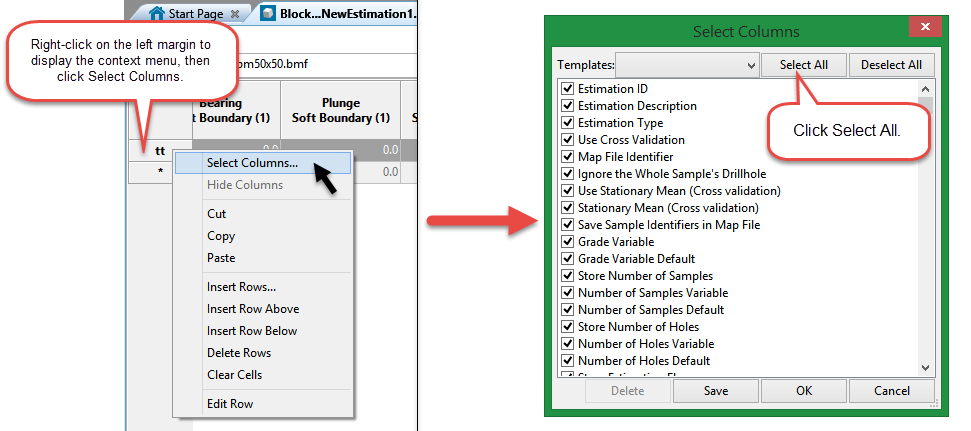
The columns are not dynamic, meaning that they will not automatically expand to include the extra cells when you enter a soft boundary count of more than 1. To get them to display, right-click on the left margin to display the context menu, then click Select Columns. In the Select Columns dialog, click Select All.
Select the variable that will be used as a criteria to identify the estimation domains.
Use the  Browse option to navigate to the triangulation. The list contains all triangulations in the current working directory.
Enter the character values that you want to ignore. To do this, click on the button to the right of the cell. A new column displays. Enter each value on a new line.
Enter the character values that you want to include. To do this, click on the button to the right of the cell. A new column displays. Enter each value on a new line.
Enter the specific values that you want to include. To do this, click on the button to the right of the cell. A new column displays. Enter each value on a new line.
Specify the value of stationary mean grade of deposit. This value is only used by the Simple Kriging estimation method.
Enter the angle clockwise from north to the bearing line. Refer to Bearing, Plunge and Dip for more information.
Enter the angle of rotation to bring the plane into the horizontal plane. Refer to Bearing, Plunge and Dip for more information.
Enter the search distance along the axis of the ore body.
Enter the search distance perpendicular to the ore body plane.
Enter the angle between the horizontal plane and the ore body axis. Refer to Bearing, Plunge and Dip for more information.
Enter the search distance in the ore body plane perpendicular to the ore body axis.
Select this check box to store the block variance, that is, the variance of a block with itself, in your block model. You will need to specify the variable in which to store the value.
Select this check box to store a flag value when a block is estimated. If a block is processed and estimated, then the flag value is stored in the flag variable. If the block is not processed, then the flag variable is not changed. If this check box is selected, then you will need to specify the variable in which to store the flag value, as well as a default flag value.
Select this check box to store the kriging efficiency in your block model. You will need to specify the variable in which to store the value. Kriging efficiency is calculated using the following formula:
(block variance - kriging variance)/block variance
Select this check box to store the kriging variance in your block model. You will need to specify a variable in which to store the kriging variance. Note that the kriging variance is not the same as the variance of your sample data. It is calculated from the variance in the variogram. If no estimate is made for a block, then the default value is written into the variance variable in the block model.
Select this check box to store the lagrange parameter. You will need to specify the variable in which to store the value, as well as a default value.
Select this check box to store the smallest kriging weight used in your block model. You will need to specify the variable in which to store the value.
Select this check box to store the number of drillholes used in the estimation for each block. You will need to specify the variable in which to store the number of holes. To use this option, each sample must have a drillhole name. Specify the database field name that contains the drillhole name.
Select this check box to store the number of samples used in the estimation for each block. The value stored will be equal to the number of samples selected prior to applying further restrictions through the Extra estimation panel.
If this check box is selected, you will need to specify the block model variable in which to store the number of samples, as well as a default value. The default value will be stored within the lock model variable when no grade estimate can be made.
If there are not enough samples to make a grade estimation, then the default value is written into the number of samples variable.
Select this check box to save the octants that were used by each estimated block.
Select this check box to save the number of octants within a nominated block model variable.
Select this check box to store the slope of regression in your block model. You will need to specify the variable in which to store the value. Slope of regression is calculated using the following formula:
(block variance - kriging variance + abs(lagrangian)) / (block variance - kriging variance + 2 abs(lagrangian))
Applicable only for folded or faulted block models for which a tetrahedral model has been created. Select the tetrahedral model. For more information on tetrahedral modelling refer to Tetra Modelling.
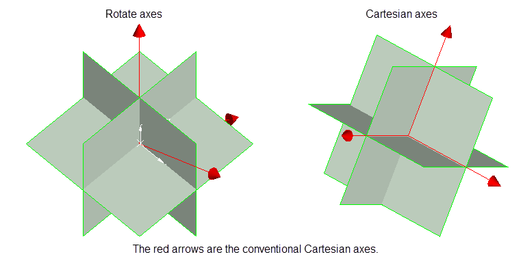
Select this check box to place a limit on the number of samples that can come from a given octant. The space around a block centre is divided into eight octants by three orthogonal planes. You have a choice of plane orientations, Rotate axes, Cartesian and Ellipsoid axes.
The Rotate axes consist of three planes perpendicular to axes that have been rotated 45° about the Z axis and 35° about the X' (X axis after rotation about the Z axis), this produces a set of planes where the first has a bearing of 135°, the second has a bearing of 45° and is at angle of -55° to the horizontal and the third also has a bearing of 45°, but is at an angle of 35° to the horizontal, see the diagram below. The Cartesian axes consist of three planes perpendicular to the conventional Cartesian axes X, Y and Z (or East, North and elevation) axes. The Ellipsoid axes consist of three planes that are perpendicular to the major, semi-major and minor axes of the search ellipsoid.
An octant search is a declustering tool used to reduce imbalance problems associated with samples lying in different directions. If there are more samples in one direction than the another, then this option limits the bias.
The samples are sorted by distance (either Anisotropic or Cartesian) prior to the samples being limited. This ensures that the closest samples are kept.
Select this check box to perform a cross validation. When performing a cross validation, the results are not written into the block model. Instead, a grade estimation is performed at each sample point while ignoring the data value at that sample point. The resulting estimates are written into a nominated mapfile for analysis. Areas where the estimated value differs significantly from the actual value may be areas that should receive extra attention. A large difference may indicate that the grade estimation process does not have enough data to provide reliable estimates.
Select this check box to limit the samples to 15 numeric fields so only samples matching certain selection criteria (specified in the Field Restrictions column) are included. Do not use spaces in the condition.
Select this check box to use median indicator kriging, which is when the same variogram model is used for each of the cutoffs.
Select this check box to limit the samples to those in a particular numeric range.
Select this option to limit the search distance to a box instead of an ellipsoid.
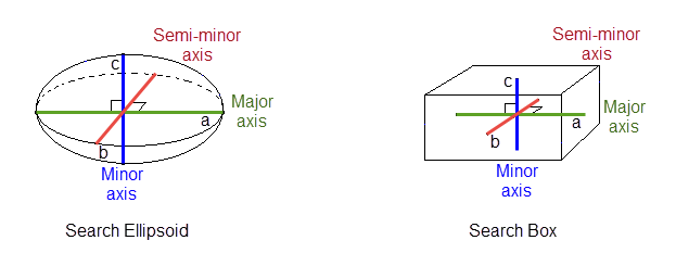
Figure 7: Search Ellipsoid/Search Box
Select this option to limit the search distance to an ellipsoid.
Select this check box to apply restricted search ellipsoids for samples that have given values of a given variable. This is commonly used to include samples from a nearby estimation domain but with restricted search radius. Sometimes samples that are at a different estimation domain share similar grade properties close to the limit between the domains. This is often known as a soft boundary between the domains. In this case, it could be useful to include samples from a different domain but only at short distances from the blocks in the current domain.
Select this check box to limit the samples to those entries that have specific character strings.
Select this check box to limit the samples to specific values in the chosen numeric field.
Select this check box to manually define the stationary mean value for the cross validation. You will need to enter the mean value through the Stationary mean (Cross validation) field.
Select this check box to manually define the stationary mean value. You will need to enter the mean grade of the deposit through the Stationary mean field. If this check box is not selected, then you can obtain the stationary mean value from a nominated block model variable.
Select this check box to multiply the sample weights by the value of the specified weighting variable. The weighting variable may represent a specific gravity, sample length or sample weight.
A block with two samples is to be estimated. The first sample has a grade value of 2 and a weight variable of 1. The second sample has a grade value of 5 and a weight variable of 2.5. The weights, from ordinary kriging, are 0.8 for the first sample and 0.2 for the second sample. Without variable weighting the estimated grade is:
(0.8 × 2 + 0.2 × 5) = 2.6
With variable weighting the estimate is:
(0.8 × 1 × 2 + 0.2 × 2.5 × 5) ÷ ( 0.8 × 1 + 0.2 × 2.5 ) = 3.15385
If the variable weighting is 0 for a block, then the default grade value is stored.
Enter the values associated with the selected soft boundary. Samples that have the values in this list for the soft boundary variable will be forced to used the ellipsoid specified in the next six fields.
Select the numeric field to which you want to limit the samples.
Select this check box to replace missing samples with zero and to use all of the weights. If this check box is not checked, then the weights of the missing samples will be ignored and the remaining weights are re-normalised to sum to 1. This option does not apply to simple kriging.

