Variogram Average

Use the Variogram Average option to calculate the average of a variogram value for a given block size.

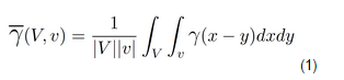
No analytical solution exists for all variogram models, so instead, the result is approximated numerically. The block is discretised in several steps (in X, Y and Z). Each discretisation point is used to evaluate the variogram model against all other points in the given block geometry.

The resulting output is displayed in the Report Window, and can be used to calculate the variance reduction factor for indicator methods, such as Indicator Kriging and Indicator Simulation, and also as an aid to defining the cell size for the block model used in Sequential Gaussian Simulation. The result may also be used in volume-variance correction and change of support models.

---

Instructions

On the Block menu, point to Simulation, then click Variogram Average.

Follow these steps:

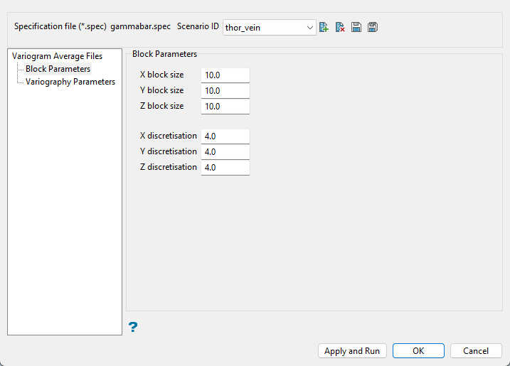
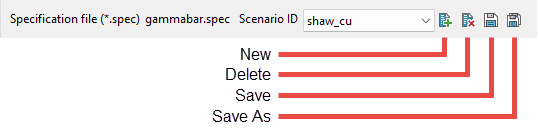
1. Select the Scenario ID from the drop-down list, or click the New icon to create a new file.

   

2. Enter the Block size. The first field is for the X direction, second for the Y direction, and third for the Z direction.

3. Enter the number of Discretisation steps for the X, Y and Z directions. The variance is obtained by discretising the block and calculating the average variogram value for all possible pairs. The X, Y, Z discretisation parameters control the number of pairs to consider. Too many points may lead to numerical precision problems. A large number of grid points can cause Vulcan to run slowly. A 4 × 4 × 4 grid is usually sufficient. In no case should there be more than 10,000 grid points.

Variography parameters

Follow these steps:

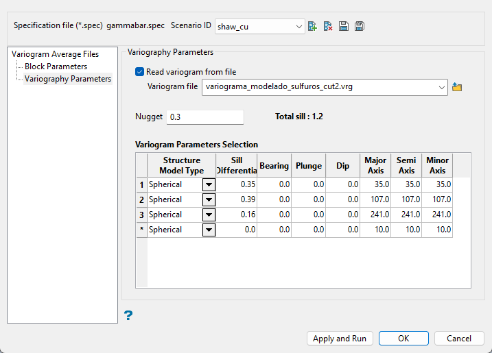
1. Enable Read Variogram from file to use an existing variogram model. The drop-down list displays all (.vrg) files found in your current working directory. Click the Browse icon to select a file from another location.

2. Enter the nugget. This represents the random variability and is the value of the variogram at distance (h) ~ 0.

3. Complete the table defining the variogram parameters to be used. Enter the information by typing into the space provided for each column.

   Explanation of table columns:

   Structure model type

   Spherical

   This type is the most commonly used for ore deposits. They exhibit linear behaviour at and near the origin then rise rapidly and gradually curve off.

   Exponential

   This type is associated with an infinite range of influence.

   The sill is reached at the specified range parameter. In release 3.2 and earlier, users were required to enter a range parameter of one-third the practical sill range. To use this model, enter the practical distance of the sill as a range parameter. For backward compatibility, see the Exponential Model 3.

   Gaussian

   This type exhibits parabolic behaviour at the origin and, like the spherical model, rises rapidly. The Gaussian type reaches its sill smoothly, which is different from the spherical model, which reaches the sill with a definite break. The Gaussian model is rarely used in mineral deposits of any kind. It is used most often for values that exhibit high continuity.

   In release 3.2 and earlier, users were required to enter a sill range of 3 times the actual sill range. To use this model, enter the effective range of the sill. For backward compatibility, see the Gaussian model 3.

   Linear

   This type is a straight line with a slope angle defining the degree of continuity.

   De-Wijsian

   This type is a representation of a linear semi-variogram versus its logarithmic distance.

   Power

   This type is computed as M - d**p where M = the maximum correlation defined as 1000.0, d = distance from the origin, p = model power. For this model type only the power p is the major axis radius. Adjust the size of the ellipsoid so that the major axis is the desired power. The size of the ellipsoid for this model does not change the calculation of the variogram.

   Exponential Model 3

   This is an un-normalised exponential model for compatibility with release 3.2 and earlier. This variogram will have the practical sill at three times the distance entered as range parameter.

   Periodic

   This is a sine wave with one complete period over the effective range. This model is not commonly used because it can cause samples at greater distances to have higher correlation.

   Gaussian Model 3

   This is an un-normalised Gaussian model for compatibility with release 3.2 and earlier. The input radius must be the effective radius multiplied by 3.

   Dampened Hole Effect

   Dampening is achieved by multiplying the covariance function by an exponential covariance, that acts as a dampening function.

   Sill Differential

   This represents the difference between the value of the variogram where it levels off and the nugget.

   Example

   If you have a total sill of 1.0, and a nugget of 0.15, you want your sill differential to be 0.85 = (1.0 - 0.15).

   

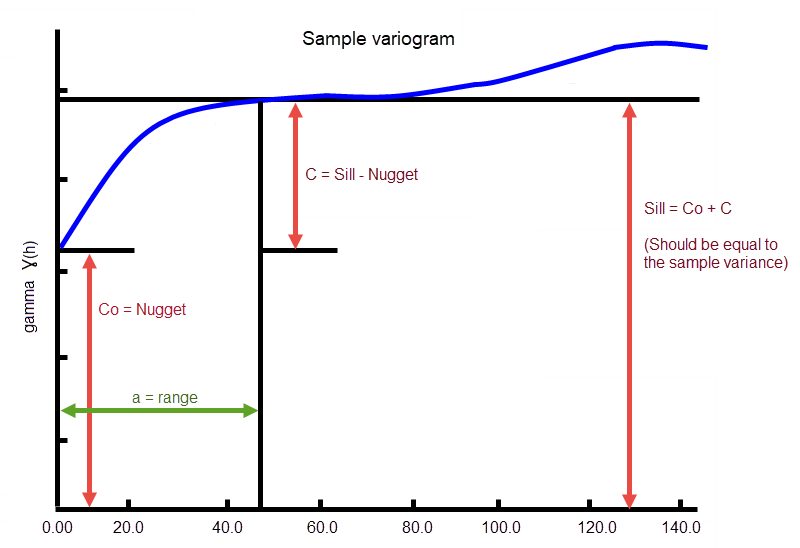
   In the diagram, C₀is the nugget, and C is the sill differential.

   Bearing/Plunge/Dip

   This is the bearing (Rotation about the Z axis), plunge (rotation about the Y axis) and dip (rotation about the X axis) of the variogram.

   Major/Semi-Major/Minor Axis radii

   This is the radii of the major, semi-major and minor axes of the variogram.

4. Click Apply and Run to save the parameters and perform the transformation.

   Select OK to save the parameters and exit the interface.

   Select Cancel to exit the interface without saving the parameters.