Load/Calculate Grid

Load/Calculate Grid is an equation (strictly speaking an 'expression') that defines a new grid to be calculated from a set of existing grids. The grid is loaded and becomes the "buffered" grid.

To display the grid as it is buffered, check the Automatically display grid check box on the Preferences panel (displayed through the Preferences option).

Note: Only one grid can be buffered at a time. Thus when you use this option the new grid replaces any existing grids in the buffer.

The expression is specified as an algebraic expression with grid names used as variables.

For example:

H.SR - H.SF

This would be read as "the H horizon structure roof minus the H horizon structure floor".

Grids can be referenced in three ways:

<mv>, for example, SF (Structure Floor)
<gfi>.<mv>, for example, C1.SF
<proj><gfi>.<mv>g, for example, ABCC1.SFG

where <proj> = the project code, <gfi> = the grid file identifier (horizon name), <mv> = model variable. In the first case, the default project and structure names are used to form a complete grid file name.

The mask value rather than the grid value may be referenced by placing a dot after the grid name, for example, if "TK." (without the quotes) is used in an equation, then the mask values of the grid TK (that is, the zeros and ones) are used rather than the TK (thickness) values.

The grid resulting from the evaluation of an expression will have an area encompassing all grids referenced in that expression, and have values determined by the expression as it is applied to grid points individually. If, while determining the value for a point, Grid Calc discovers that the point falls outside the geographic area associated with one of the grids, then the contribution from that grid is a zero (this occurs in the case where the data being manipulated cover different geographical areas).

The mask values are ignored when determining the new grid values, but they are used to determine the mask for the new grid. By default, the grid mask at a given grid location is determined by the 'intersection' (logical AND) of all mask values for all grids referenced in the expression for that point. If a point falls outside any of the grid areas referenced, then the mask for that point is taken to be zero (off). If the masking mode is set to OR, then the resulting mask for grid points is the union (that is, logical OR) of all masks for all grids referenced in the expression. See the Project Defaults option with regards to the Masking Modes parameter.

See the Mask Function for further information on mask node values.

If literal values (for example, 190.23, 1, 232, etc.) are referenced in an expression (for example, 100*TK), they correspond to grids of constant value. An expression cannot be made up of constant values alone, unless a grid is buffered. Obviously, a constant value does not define a geographic region so the grids in the equation (or the buffered grid) are used to define the area.

The following operators may be used in an expression:

Binary Operators	-, *, /, ^
Logical Operators	or, and, xor, not, le, ge, lt, gt
Functions	sin(x), cos(x), tan(x), asin(x), acos(x), atan(x), abs(x), sqrt(x), xp(x), ln(x), log(x), frac(x), int(x), min(a,b,c,...), max(a,b,c,...), mod(n,m), sgn(x), mask(eqn)

Logical and numeric operators may be combined in an expression. A logical expression evaluates to 0 (false) or 1 (true). This allows logical operators to be used to form IF type expressions.

For example, if you desire to set a thickness grid (TK) to zero wherever it has a value less than or equal to 0.5 then the following expression could be used:

tk*(tk gt 0.5)

The sub-expression in brackets "tk gt 0.5" evaluates to 1 (true) every time the TK grid has values greater than 0.5. Elsewhere, it evaluates to zero.

In addition to grids, the following variables may be referenced in an equation:

x, y, z, dip, dir(q), bear, g(i,j), r(x,y)

These 'standard variables' make use of the buffered grid. They represent values derived from that grid. The variables are determined each time the expression is evaluated at a grid node. The variables x, y and z, evaluate to the current easting, northing and z value. The dip is the dip of the surface at the location being evaluated. The dir (q) is the acute angle of the dip from the specified angle. If no angle is specified, then a default angle of zero (North) is used. Angles are specified in bearings from North (in radians). Negative angles are accepted. All angles returned by dir are in the range zero to π (180 degrees). bear is the bearing from North of the dip direction. It differs from dir(q) in that the angle returned in radians is a value between 0 and 2π (360 degrees). The functions g and r are similar. They return the z value for the point offset from the current point by the amount specified. The offset for g(i,j) are specified in terms of grid cells, while r(x, y) accepts actual distances.

After generating a new grid, save it using the Save command. You can perform the save step at the same time as the calculation by using the following command (entered in the command line):

grid=equation

For example, the following generates a thickness grid by subtracting a structure roof (SR) grid from a structure floor (SF) grid:

tk=sr-sf

Instructions

On the Grid Calc menu, point to Grids, and then click Load/Calculate Grid to display the Load/Calculate panel.

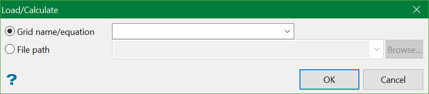
Grid name/equation

Enter the grid equation. The drop-down list contains all of the grids found in your current working directory.

File Path

You can browse to load/calculate grids from other directories.

Note: If no equation is specified and the grid name alone is entered, then the option works as an Open command for that grid.

Click OK.

The new grid will be buffered.

To display the grid, use the Static Display Grid or Dynamic Display Grid options (under the Grid Calc > Display submenu). You can also type one of the following two commands at the Grid Calc command line:

plot plot_grid