Model
Use the Grid Model option to generate a grid model from the loaded data points.
We recommend that you monitor the modelling process through the Grid Calc Report Window. Information about the data and the model are displayed in this window and can be saved and printed by using the appropriate icons.
Instructions
On the Grid Calc menu, point to Model, and then click Grid Model to display the Model Select panel.
Your choice of the method will determine which options (in the next panel) can be used. If an option is shadowed, then it is not applicable to your chosen method.
Triangulation (linear triangulation)
The Linear Triangulation method is typically used for modelling structural surfaces, such as structure roof and floor and structure thicknesses, and is recommended for modelling deposits with thin bedding planes. The results are a unique interpolated surface that honours all of the raw data values. Using a Trend Surfacewith this modelling method allows a regional feature to be applied to the local area of interest. TheSmoothingoption can be used to relax the triangle facets for a smooth grid and nicer looking contours.
The triangles are as close to equilateral as possible and have a data point at each vertex. There will be linear interpolation between the three node points that make up each triangle. This method cannot extrapolate values higher or lower than the actual point values, causing the tops of hills and the bottoms of drainage areas to become flat. To avoid this scenario, the triangulation can be manipulated by applying a spline to the surface. The triangle network is covered with a mathematical surface that passes through each data point and is tangential to each point's previously determined slope, resulting in a surface that changes smoothly in all directions. All of the raw data values are honoured and the surface is projected above and below raw data values between data point locations.
This method allows for surface extrapolation beyond the raw data point locations. Vulcan uses Trending and Inverse Distance to extrapolate a triangulation to the model's edge.
Inverse distance (average weighting)
The Inverse Distance Weighting method is typically used for modelling thickness and quality information. This method searches concentrically about each grid node for a minimum number of points to use to interpolate the grid node value. The number of points (NOIP) used and the distance to search for these points is specified as part of the method parameters. You can also divide the area into a maximum of 8 sectors, forcing the program to find the closest points in each sector, which is useful if the drillhole data is predominantly found in one section of the modelling area.
This method should not be used on faulted datasets or for deposits where the bedding planes are thin.
The grid node values are determined by taking a weighted average of the collected data points. Therefore, the closer a drillhole is to the grid node, the greater the effect it will have on the calculated node value. The weighting used is the inverse of the distance to the nominated power (the default value is 2).
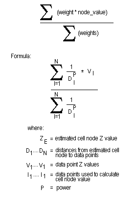
Figure 1: Inverse Distance Calculation
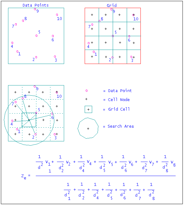
Figure 2: Inverse Distance Example
Krige (statistical analysis)
The Krige method is based on a statistical analysis of spatially located data. The first step in kriging is to perform a variography analysis of the sample data. The resulting variograms express the degree of correlation between samples as a function of distance in several different directions. Sample data are usually correlated at short distances and less correlated at longer distances. Some sample data, such as water table levels, show a high degree of correlation at short distances. Other sample data, such as gold grade, usually show a larger degree of variance even at short distances. All sample data show a correlation approaching zero at larger distances. By fitting a variogram model function to the correlation data we make a function that predicts how well two samples will be correlated given their spatial relationship.
This method estimates a variable at a point by locating and weighting nearby samples. The weights take into account the degree of correlation between each sample and the estimation point, and also the degree of correlation between each pair of samples. The resulting weights provide a de-clustered weighting of the samples that minimises the variance as defined by the variogram.
Spline surface (flexible curve)
The Spline surface (flexible curve) method uses a drafter's spline, which is a flexible curve that can be fitted to a sequence of points so that a smooth curve can be drawn between them. The procedure fits a low order polynomial along the grid lines to all adjacent sets of points and from these it interpolates values at the grid points. The spline method demands that the data points lie on the grid lines where the X and Y values are multiples of the grid spacing. Normally, the spline method is used to model string data, such as contours. The strings should be loaded into Grid Calc using the Use slice option on the Data > Load Design option. The tension of the splines may be specified (negative value implies relaxed) as can the bias applied to the splines in the X (vertical bias) and Y (horizontal bias) directions.
Least squares (best fit)
The Least squares (best fit) method is sometimes called a "moving average" because each node in the grid is estimated as the average of values from control points in a neighbourhood that is "moved" from grid node to grid node. First, all control points are located that reside in a specified neighbourhood around the grid node to be estimated. The values of these points approximately define a sloping plane or low order polynomial. Secondly, the equation of the plane is calculated and used to estimate the value of the grid node. The process of fitting a plane and evaluating it to estimate the surface is repeated for every node on the grid.
Trend surface (applying the shape of the regional geology)
The Trend surface method is based on the premise that small-scale features are masked and distorted in maps that are dominated by large scale, high amplitude features. Consequently, if the large-scale features are removed, then the smaller features are more easily identified and evaluated. This method applies a specified regional trend to the modelling process and then to evaluate the residuals, or differences between the raw data values and the regional geological trend of the area.
First, a smooth regional map called a "trend surface" is made, this is a two dimensional global polynomial function. Then the differences between the original data point values and the smooth regional trend are calculated to produce a "residual" map (which displays the local features). Both maps may be significant in the geological interpretation.
Polynomials of degree 1, 2 and 3 are known as linear, quadratic, and cubic polynomials. A polynomial of degree 1 is a straight line if it is two dimensional or a plane if it is three dimensional. Every polynomial of degree 2 is a parabola with a vertical axis of symmetry that represents an anticlinal or synclinal shape. A third order polynomial defines an undulating surface. The third order trend may be applied to regional areas where both an anticline and an adjacent syncline are present or regions where the strata is actually folded. Higher order polynomials are not representative of geological surfaces. They tend to oscillate wildly between the outside control points and may generate very distorted values near the model's edge. How well the surface statistically fits the data can be determined from the "Goodness-of-fit" information produced during the modelling process.
User defined
Select the Method name from the drop-down list. This to access any customised modelling methods previously set up through the Define Method option (under the Grid Calc > Edit Modelling Defaults submenu). If you have chosen to apply the horizon table crop layer as the mask (when defining the method), then the name of the crop layer displays on the panel.
Click OK to display the Model panel.
Setup tab
Method
The modelling method displays in this section it cannot be overwritten.
Alternate Coordinate Window
Select this check box to enter the geographical extent of the grid in X and Y coordinates. It is not necessary to specify the extents. The default window generated or defined at the time the data points were loaded is used if no extents are specified. If you do specify the extents, then they are added to the replay.gdc_cmnd macro file.
Grid size
Enter the grid size of the generated model. If a grid size is not specifed, then the default grid size generated or defined at the time the data points were loaded will be used instead.
Trending order
Specify the trending order (as an integer). This converts the data to residuals before the modelling step, and then adds back the trend after modelling.
Smoothing passes
Specify the number of smoothing passes to be applied to the grid once it has been created. Smoothing applies a mathematical equation that calculates the variance of the modelled data. Once the value has not changed from the previously calculated variance by a certain percentage, the iterations or calculation process are discontinued. Usually nine smoothing passes are sufficient.
Options tab
The method you have chosen determines which options on this panel will be available to you. Refer to the documentation below for information on the options that are applicable to your choice of method.
|
Method |
Options |
|
Triangulation |
|
|
Inverse Distance |
|
|
Krige |
|
|
Spline |
|
|
Least Squares |
|
|
Trend Surface |
|
|
Modelling Method and Parameters |
|
|
Spline surface |
Select this check box if you want to produce smooth grids without any smoothing when interpolating within the triangles. Breaklines are recognised. |
|
Maximum triangle side length |
Enter the maximum length for a triangle side. Grid points evaluated within a triangle with a side length greater than the specified length will have a data mask value of " |
|
Inverse distance power |
Enter the inverse distance power (the default value is " |
|
Maximum number of points |
Specify the number of interpolative points to be used by the inverse distance method (the default value is " |
|
Maximum search distance |
Specify the maximum search radius for the inverse distance method. Grid points evaluated using points further than this distance from the grid point will have a data mask value of zero. The default is unlimited search distance. |
|
Number of search sectors |
Enter the number of search sectors (a maximum of " |
|
Sector angle offset |
Enter an angle, in degrees, for the offset of the sectors. For example, if you choose to have 6 sectors and a sector angle offset of 0°, then the first sector extends from a bearing of 0° to a bearing of 360 ÷ 6 (360 divided by 6)=60°. However, if the number of sectors is 6 and the sector angle offset is 5°, then the first sector extends from a bearing of 5° to a bearing of 60+5=65°. Rotating the sectors can stop samples being located on a boundary, which can cause problems as there is no way to determine into which sector a sample is placed if it is on a border. |
|
Vertical bias |
Enter the bias to be given to splines along the vertical grid lines over the horizontal grid lines. For each grid point, two values are interpolated, one based on the vertical spline, the other on the horizontal spline. The actual grid value is determined by averaging these values. The VERTICAL BIAS and HORIZONTAL BIAS values are used to weight the average vb/(hb+vb) and hb/(hb+vb). |
|
Horizontal bias |
See Vertical bias for an explanation. Note: For no bias, leave both the Vertical bias and Horizontal bias fields blank. To ignore one or the other, use 1 and 0 or 0 and 1 (if Horizontal bias is zero, then the horizontal splines are ignored). To give twice as much bias to the vertical splines as to the horizontal splines, use Vertical bias 2 and Horizontal bias 1. Multiplying the bias by a value has no affect, i.e. 2 and 1 is the same as 20 and 10. If you are modelling contour data, and most contours run East/West, you will want to use a high Vertical bias since the splines running North/South will have lots of control from the contour, while those running East/West will be almost parallel to the contours and hardly ever intersect them. |
|
Spline tension |
Enter the spline tension. A negative value relaxes (curves) the splines, therefore the higher the negative value the more relaxed the splines will be, that is they curve more. A positive value increases the spline tension, it makes the splines pull tight over the control points, reducing, for example, the height of the tops of hills and the depth of valleys. The values are usually in the range of -3 to 3, but they can be more or less. |
Krige tab
The method that you have chosen determines which options are available to you. For the Krige method all of the options are available.
Model name
Select one of Spherical, Exponential and Gaussian as the variogram model type.
Nugget of variogram
Enter the standardised nugget value returned from variogram analysis. The value returned (between 0 and 1) is the proportion of the variogram model sill represented by the variogram model nugget.
If the variogram model nugget value is '0.4', and the variogram model sill value is '2.0', then the nugget entered will be 0.4 ÷ 2.0 = 0.2.
The sill value does not need to be entered as its standardised value will be set as '1'.
The following fields define the shape and size of the variogram.
Bearing to major direction
Enter the bearing of the major axis of the ellipse.
Major range to the sill
Enter the length of the major axis. This is the distance from the centre of the ellipse to its edge in the major direction.
Minor range to the sill
Enter the length of the minor axis. This is the distance from the centre of the ellipse to its edge along the minor axis. The minor axis is perpendicular to the major axis.
If bearing = 90, major = 25 and minor = 15, then the ellipsoid is 50 long in the East/West direction, 30 wide in the North/South direction, and the major axis is parallel to the East/West axis.
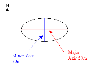
Figure 3: Example ellipse
If the bearing = 0, major = 25 and minor = 15, then the ellipsoid is 50 long in the North/South direction, 30 wide in the East/West direction, and the major axis is parallel to the north-south direction.
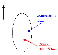
Figure 4: Example ellipse
Click OK.
The points are then modelled.

