Strategic Designer
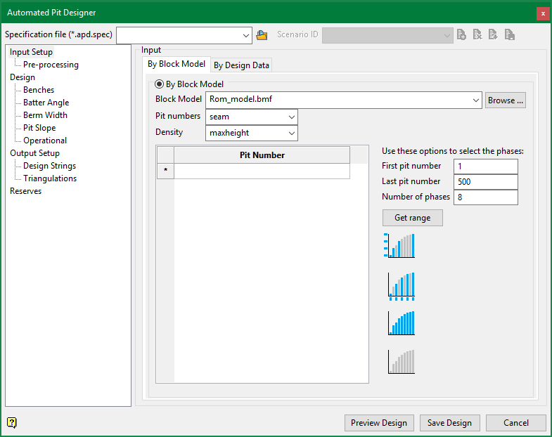
The Automated Pit Designer in Vulcan allows you to create an open pit design directly following pit optimization. It uses either pit numbers from a given block model or design data, in the form of closed polygons, to automatically project benches and offset at appropriate operating widths to create high level operational pit designs.
On the Open Pit menu, point to Automated Pit Designer, then click Automated Pit Designer.
The automated pit designer is divided into the following main sections
Input Setup
This section defines the input data which will form the basis for the pit designs. Input may be read directly from a block model, or supplied as user digitized polygons.
Design
This section defines the geotechnical and operational parameters which dictate the shape of the resulting pit. Batter angles, berm widths, and minimum mining width are a few of the settings defined in this section.
Output
This section defines the results. The results from the pit designer may be saved to a layer as design strings or triangulated for reserving and scheduling.
There is a toolbar along the top of the panel to manage multiple specification files and multiple scenarios within those spec files.
-
Use the Browse button or the combobox to create or select an existing specification file.
-
Use the Scenario Selector to switch to a different scenario. If unsaved changes exist you will be asked to save your current changes, or confirm the switch thereby discarding any changes.
-
Use the New Scenario button to create a new blank scenario. You must specify a unique name for the new scenario.
-
Use the Delete Scenario button to delete the current scenario. You will be asked to confirm the deletion.
-
Use the Delete Multiple button to delete multiple scenarios at a time. You will be asked to confirm the deletion.
-
Use the Save as button to save the current scenario as a different scenario.
-
Use the Save button to save the current scenario.
There are three buttons along the bottom of the panel.
-
Select Preview Design to preview the design on screen as an underlay.
-
Select Save Design to save the design into the layer specified in the Output setup section. This will also triangulate the designs if requested.
-
Select Cancel to close the panel without saving.
Specification file (.apd.spec)
Use the drop-down list to select the specification file if it is in the current working directory, or browse for it in another location by clicking the Browse button. You may also create a new file by typing the name of the new file in the textbox.
-
 Browse
Scenario ID
A scenario is a set of parameters that is used to build one specific (.apd.spec) file. You can copy an existing scenario and save it to a different name, modifying it as desired, or create a new scenario.
-
 New
New -
 Delete
 -
 Save as
 -
 Save
Save
Buttons along the bottom of the panel.
Preview Design
Preview the design on screen as an underlay.
Save Design
Save the design into the layer specified in the Output setup section. This will also triangulate the designs if requested.
Cancel
Close the panel without saving.
This section is used to define various optional parameters to preprocess the data before the automated pit design process. All of these parameters are optional, but can help to ensure the automated pit designer creates a valid design.
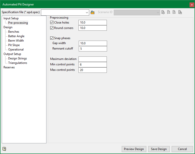
Close Holes (Closing) / Round Corners (Opening)
These parameters are used to preprocess the input in order to remove small asperities, isolated blocks or other issues in the input. Each parameter is supplied in distance units. These operations will be applied to the block model, or the design data. Although slightly different (conceptually identical) algorithms are used for design data than those described here.
With block model input, the element radius is supplied as a real distance, but it is translated into a binary structuring element based on the underlying parent block size. An element radius less than the parent block size will have no impact.
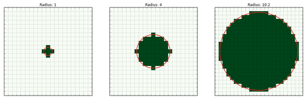
Figure 1: Structuring element by supplied radius. This block model has 1m x 1m blocks.
The Morphological Closing will expand (dilate) the input shape based on the structuring element and then contract (erode) the shape. This will remove isolated holes, join shapes together and in general ‘close’ the input model.
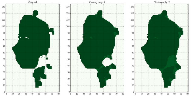
Figure 2: Closing by example. A single bench in plan, original uncleaned pit optimisation results on the left, Closing with an element of size 4 and 7 in the middle / right respectively.
The Morphological Opening will contract (erode) the input shape based on the structuring element and then expand (dilate) the shape. This will remove isolated blocks and sharp interior corners.
Often, both the closing and the opening should be used in tandem:
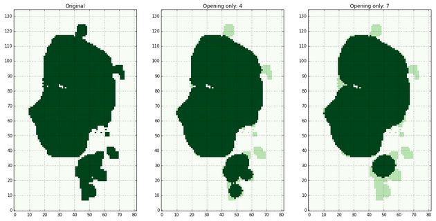
Figure 3: Opening by example. A single bench in plan, original uncleaned pit optimisation results on the left, Opening with an element of size 4 and 7 in the middle / right respectively.
These options can be used to enforce minimum mining width prior to generating the design. Also note that minimum mining width can also be set explicitly in Design > Operational.
Snap Phases
When block model input is used it is useful to snap earlier phases to later phases. This helps enforce a reasonable mining width between phases.
The Gap Width is supplied in distance units. It is converted into a structuring element as above, and then used to selectively snap inner phases to outer ones.
The Remnant Cutoff is a cutoff in number of blocks below which 'remnants' will be set to the earlier phase. A Remnant is a small section of blocks which is both along the edge of the later phase and is surrounded by the inner phase. For example in Diagram 4 below there are three remnants. Along the top near 100, 145, on the right side at 135, 90 and at the bottom near 100, 45. The topmost remnant would be included in the inner phase if a large enough remnant cutoff was specified.
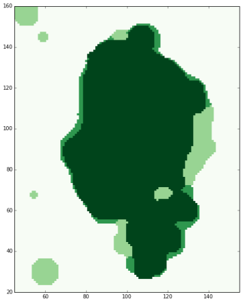
Figure 4: Example of snapping phases. The innermost dark green blocks are phase 1. The outermost light green blocks are phase 2. The green blocks between them are the result from snapping with a radius of 3 blocks and a remnant cutoff of 20.
Maximum Deviation
Use this parameter to control the maximum deviation of the seed shapes, which are used to create the pit design, from the input shapes that were specified in Input Setup. This deviation is measured from each point to the seed shape. This parameter is supplied in distance units.
When block model input is used, this parameter will default to the diagonal distance across a parent block divided by two which has, in practice, lead to acceptable pit designs. When using contours from a block model, it is not recommended to set the deviation to 0. When design data input is used, this parameter will default to 0, however this should be carefully tuned based on the character of the input polygons.
This deviation should either be set to 0, in which case the points are interpolated, or set to a medium sized number (relative to the distance between input points) in which case the shape is fit by least squares. If a very small deviation is used the least squares fitting will exhibit Runge’s phenomenon and lead to very unstable pit designs. Note, this deviation may not be honoured due to reaching the maximum number of control points.
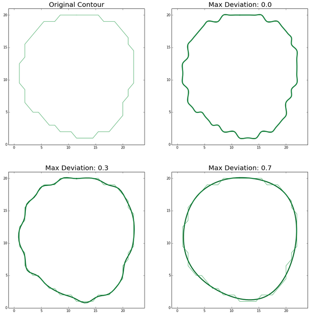
Figure 5: The effect of the maximum deviation.
Min Control Points / Max Control Points
Each pit contour or design boundary is described by relatively few control points. You may specify a minimum and maximum number of control points which can help in fitting the input data. These options are only available if the maximum deviation is greater than 0, because if the deviation is 0 a different interpolation algorithm is used.
A large number of control points is not suggested, as Runge’s phenomenon may occur. Using a large number of control points may also increase the computation time.

Figure 6: Runge’s phenomenon. Using too many control points (line in blue) will have lower deviation (distance from input points), but much greater deviation from the character of the line. The green line uses less control points with a higher deviation, but fits the data better.
This section contains the default design parameters which controls the projection of the polygons from bench to bench. Optional advanced parameters for each measure can also be specified in the child panels.
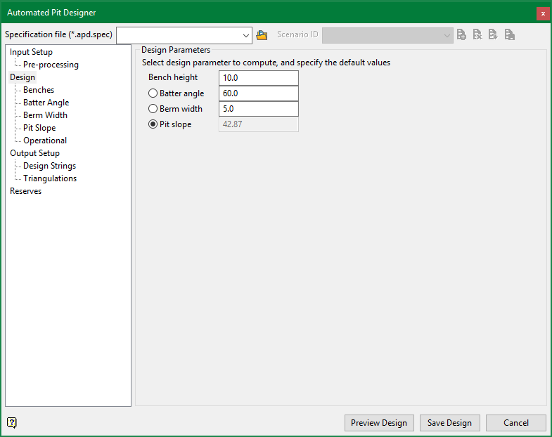
Refer to Diagram 1 for a visual representation of the design parameters in cross section.
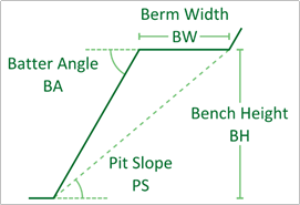
Figure 7: Schematic for Design Parameters
The bench height must be set, and then any two of the three remaining parameters may be specified. The fourth will be calculated from the other three.
Bench Height
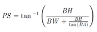
Enter the default bench height. For reference, the bench height in terms of the berm width, pit slope and batter angle is given by the following relation:
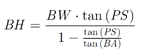
This quantity is entered in distance units.
Batter Angle
If Calculate Batter Angle is selected; the box to enter the default batter angle will be greyed out and the batter angle will be calculated using the following equation:
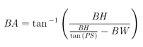
This quantity is entered in degrees.
Berm Width
If Calculate Berm Width is selected; the box to enter the default berm width will be greyed out and the berm width will be calculated using the following equation:
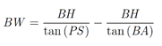
This quantity is entered in distance units.
Pit Slope
If Calculate Pit Slope is selected; the box to enter the default pit slope will be grayed out and the pit slope will be calculated using the following equation:
This quantity is entered in degrees.
Note: Advanced parameters are not available for the quantity that is calculated, as this could lead to an overdetermined problem. Also, advanced parameters will always overwrite default values, unless they are invalid.
This section contains the advanced bench height parameters. Note: All elevations in this panel are toe elevations. Currently, only flat benches are supported.
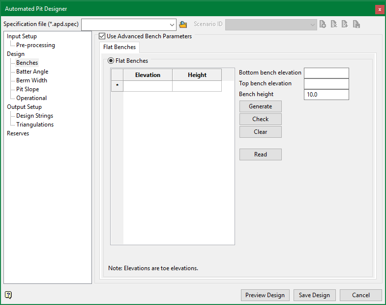
Use the grid to enter the toe Elevation and bench Height. If double benching, it is acceptable to delete a bench and double the height of the bench below.
Instead of entering the elevation and height information manually you may optionally use the Bottom Bench Elevation, Top Bench Elevation, and Bench Height boxes with the Generate button to populate the grid. The Bottom bench elevation will be preferred over the top bench elevation if they do not line up.
Use the Check button to ensure that the entered elevations and heights are valid. The elevations and bench heights must cover the entire vertical extent of the pit. This should be used if the benches are entered manually. For example, a toe elevation of 5 with height 10 must be followed by a toe elevation of 15. Note that the benches can extend above the model.
The Read button can also be used to calculate the benches automatically from the input block model. This will read the block model, and based on the phases specified in the Input Setup grid determine the lowest and highest blocks. Benches are then generated between these two elevations using the Bench Height in this panel.
Benches may extend above or below the input data.
This section contains the advanced batter angle parameters. Batter angles may be supplied in two main ways.
By Block Model
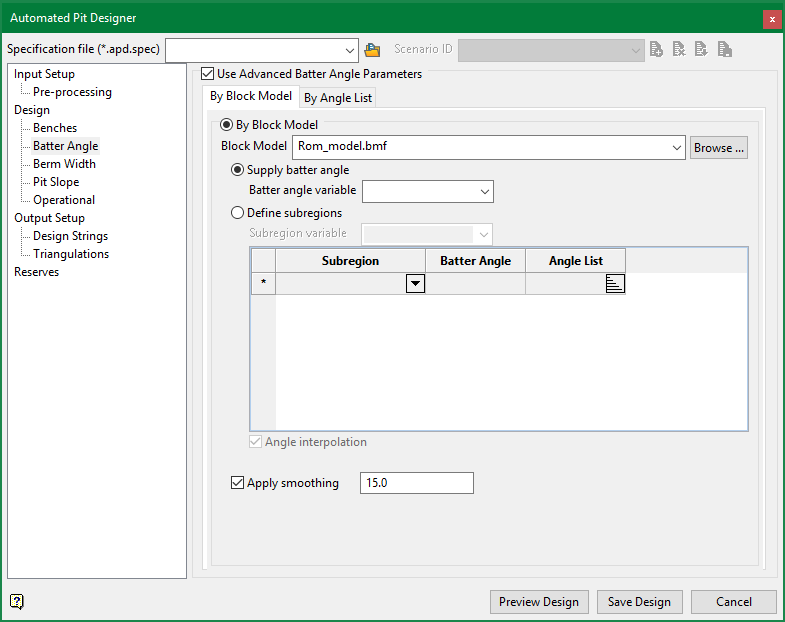
The first way to supply the batter angles is from a block model. First, specify the Block Model which contains the batter angle information from the drop-down or browse to a block model in a different location. Once the block model is selected there are two ways to supply the Batter Angle Information. Note: This block model does not need to be the same as the pit number block model, it could even be a different size, which could improve computation time.
Supply Batter Angle
Use this option to supply the Batter Angle Variable as a numeric block model variable. This quantity is entered in degrees.
Note: Values below 0.5 degrees or above 90 degrees are set to the default batter angle.
Define Subregions
Use this option to elect an integer or name type Subregion Variable which specifies several subregions or domains.
If the subregion variable is a name type variable you may select the Subregion from the drop down menu. If the subregion variable is an integer type variable enter the value for each subregion in the Subregion column.
Then, use the rest of the grid to enter either the Batter Angle for each Subregion or specify an Angle List. An example angle list is shown below.
Note: The angle list will overwrite the Batter Angle in the second column
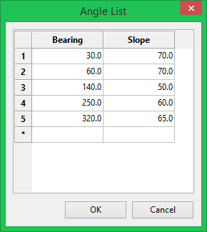
Figure 8: Angle List Grid Panel with example input.
Enter the Bearing for each Slope angle. At each bearing the slope will be reproduced precisely. You can optionally apply linear interpolation between the angle by selecting the Angle Interpolation checkbox. For the example Angle list specified in the panel above the slope angles used for all bearings with and without linear interpolation are shown in Diagram 1 below.
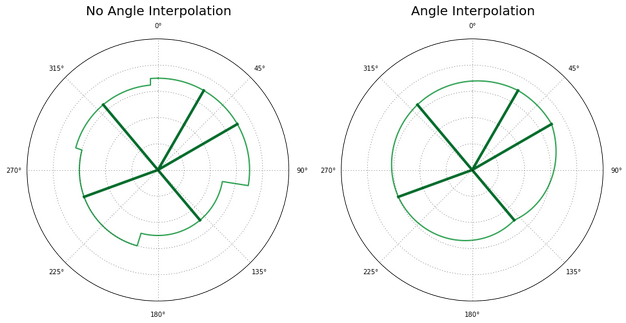
Figure 9: Schematic for angle interpolation. Without angle interpolation the nearest bearing is used.
Note: Any subregions without an associated batter angle or angle list will revert to the default batter angle. Any inappropriate values (such as -99s) will also revert to the default batter angle.
Apply Smoothing
Use the Apply Smoothing option to ‘smooth’ the batter angles across boundaries. The quantity is supplied in distance units and is measured along the polygon which is to be projected.
Refer to Diagram 2 for a small example. Note that the angle to project at is based on the polygon which is being projected – this is why the offset in the 60 degree region is not aligned with the block boundary, the transition between 70 and 60 degrees occurs at the interior polygon.
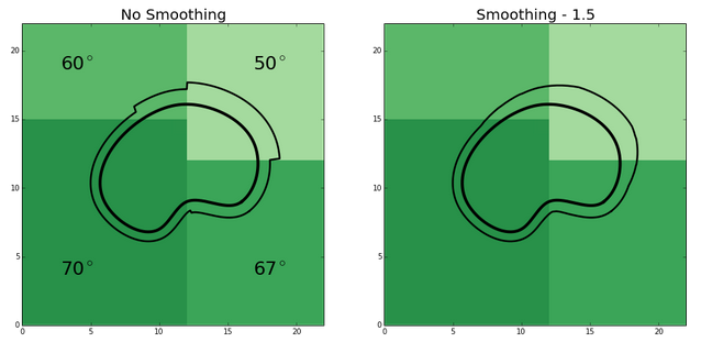
Figure 10: Schematic for block model smoothing. The thick black line is the toe, the thin black line is the projected crest. The underlying block model is coloured by batter angle.
By Angle List

The second way to define the batter angle is with a single angle list. This angle list will apply to all locations. Enter the Bearing for each Slope angle. At each bearing, the slope will be reproduced precisely. You can optionally apply linear interpolation between the angle by selecting the Angle Interpolation checkbox.
Refer to Figure 1, above, for an example of what Angle Interpolation will do.
Apply Smoothing
Use the Apply Smoothing option to ‘smooth’ the batter angles across boundaries. The quantity is supplied in distance units and is measured along the polygon which is to be projected.
This section contains the advanced berm width parameters.

The first way to supply the berm widths is from a block model. First, Specify the Block Model which contains the berm width information from the drop-down or browse to a block model in a different location. Once the block model is selected there are two ways to supply the Berm Width information. Note: This block model does not need to be the same as the pit number block model.
Supply Berm Width
Use this option to supply the Berm Width Variable as a numeric variable. This quantity is entered in distance units. Note: Values below 0.0 are set to the default berm width.
Define Subregions
Use this option to elect an integer or name type Subregion Variable which specifies the subregion or domain.
If the subregion variable is a name type variable you may select the Subregion from the drop down menu. If the subregion variable is an integer type variable enter the value for each subregion in the Subregion column.
Then, use the rest of the grid to enter either the Batter Angle for each Subregion
Use the Apply Smoothing option to ‘smooth’ the batter angles across boundaries. The quantity is supplied in distance units and is measured along the polygon which is to be projected.
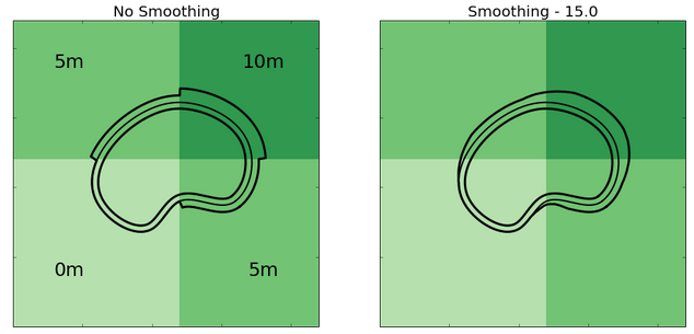
Figure 11: Schematic for block model smoothing. The interior thick black line is the lower bench toe, the thin black line is the crest, the exterior thick black line is the offset toe. The underlying block model is coloured by berm width.
This section contains the advanced pit slope parameters. Pit slope may be supplied in two main ways.
By Block Model
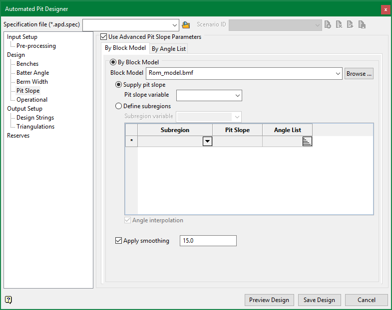
The first way to supply the pit slope is from a block model. First, specify the Block Model which contains the pit slopoe information from the drop-down or browse to a block model in a different location. Once the block model is selected there are two ways to supply the Pit Slope Information. Note: This block model does not need to be the same as the pit number block model, it could even be a different size, which could improve computation time.
Supply Pit Slope
Use this option to supply the Pit Slope Variable as a numeric block model variable. This quantity is entered in degrees.
Note: Values below 0.5 degrees or above 90 degrees are set to the default pit slope.
Define Subregions
Use this option to elect an integer or name type Subregion Variable which specifies several subregions or domains.
If the subregion variable is a name type variable you may select the Subregion from the drop down menu. If the subregion variable is an integer type variable enter the value for each subregion in the Subregion column.
Then, use the rest of the grid to enter either the Pit Slope for each Subregion or specify an Angle List. An example angle list is shown below.
Note: The angle list will overwrite the Pit Slope in the second column
Figure 12: Angle List Grid Panel with example input.
Enter the Bearing for each Slope angle. At each bearing the slope will be reproduced precisely. You can optionally apply linear interpolation between the angle by selecting the Angle Interpolation checkbox. For the example Angle list specified in the panel above the slope angles used for all bearings with and without linear interpolation are shown in Diagram 1 below.
Figure 13: Schematic for angle interpolation. Without angle interpolation the nearest bearing is used.
Note: Any subregions without an associated pit slope or angle list will revert to the default pit slope. Any inappropriate values (such as -99s) will also revert to the default pit slope.
Apply Smoothing
Use the Apply Smoothing option to ‘smooth’ the pit slopes across boundaries. The quantity is supplied in distance units and is measured along the polygon which is to be projected.
Refer to Diagram 2 for a small example. Note that the angle to project at is based on the polygon which is being projected – this is why the offset in the 60 degree region is not aligned with the block boundary, the transition between 70 and 60 degrees occurs at the interior polygon.
Figure 14: Schematic for block model smoothing. The thick black line is the toe, the thin black line is the projected crest. The underlying block model is coloured by pit slope.
By Angle List

The second way to define the pit slope is with a single angle list. This angle list will apply to all locations. Enter the Bearing for each Slope angle. At each bearing, the slope will be reproduced precisely. You can optionally apply linear interpolation between the angle by selecting the Angle Interpolation checkbox.
Refer to Figure 2, above, for an example of what Angle Interpolation will do.
Apply Smoothing
Use the Apply Smoothing option to ‘smooth’ the pit slopes across boundaries. The quantity is supplied in distance units and is measured along the polygon which is to be projected.
This section contains the operational parameters which control the shape and character of the final pit design. All of the parameters in this panel are optional.
Minimum Mining Width
Minimum mining width is defined as an effective diameter within which equipment can operate. Any areas of the pit which do not satisfy this mining width are re-designed to satisfy this constraint. Refer to Diagram 1 for a schematic of the minimum mining width. This quantity is supplied in distance units. The default is 0.
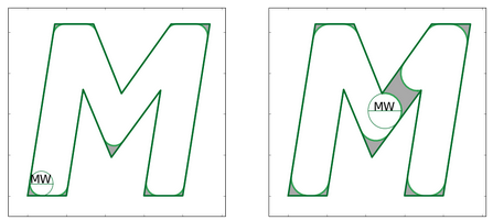
Figure 15: Schematic for Minimum Mining Width. The dark green polygon is slated for extraction, however with the given minimum mining widths the grey shaded regions are unmineable.
This is applied to the input, and is functionally identical to the input processing round corners.
Minimum Outer Radius
This parameter is an effective outer radius that the bench must satisfy. This is in place to allow control over “noses” or other concavities which may occur. Refer to Diagram 2 for a schematic of the minimum outer radius. This quantity is supplied in distance units. The default is 0.
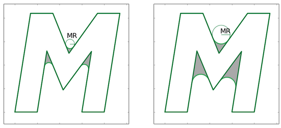
Figure 16: Schematic for Minimum Outer Radius. For enforcing the outer radius. The dark green polygon is slated for extraction, however with the given minimum outer radii the grey shaded regions must be mined as well.
The Minimum Outer radius is measured with respect to the toe. Therefore this radius may be violated by the crest lines. If the expected planar distance between the toe and the crest is constant this distance could be added to the radius to enforce the outer radius of curvature in the crest lines.
This quantity may also be used to enforce a minimum flat width, again note that this radius is measured from the toe. This form of using the minimum outer radius is shown in Diagram 3 below.
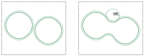
Figure 17: Schematic for Minimum Outer Radius. For enforcing a minimum flat width. On the left; a minimum outer radius of 0 is specified, and the toes (thick green lines) project to crests (thin green lines) that are very close together. With a minimum outer radius as specified on the left, the polygons will be joined together prior to projection.
Minimum Area Delta
This parameter is used to limit ‘delamination’ of the pit design. If the local area delta of the input shapes on a given bench to the projection from the lower bench is less than this quantity the given bench will snap to the lower bench. The parameter can be visualized with the following schematic.
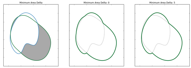
Figure 18: Schematic for minimum area delta. The lower berm is shown in blue, the toe from the input polygon in green. The area of the gray regions is evaluated. The effect of the minimum area delta is shown in the middle and on the right.
The lower bench berm is shown in blue, the toe from the input polygon in green. The area of the two gray regions will be evaluated, if the area of either region is less than the minimum area delta the respective region will be discarded. In this particular example it is reasonable to discard the very slight area in the upper left. An appropriate minimum area delta will achieve this.
This quantity is supplied in distance units squared. The default is 0.
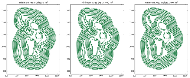
Figure 19: Effect of minimum area delta on a pit design. As the minimum area delta increases, the pit design ‘snaps’ together, towards the pit bottom.
The automated pit designer progresses upwards, from the lowest bench to the highest. At each bench it will take the projected result from the bench below, lets call these 'projected polygons', and the input polygons from the block model, the 'input polygons'. Both the projected polygons and the input polygons represent the outer boundary of the desired pit. They both should be honoured. If only the projected polygons were honoured only the lowest input polygons would be used. This may be simulated with a very large minimum area delta. In only the input polygons were honoured it would not look like a pit, and would defeat the purpose of this option.
Therefore, there are two answers at the base of any given bench - The projected and bermed polygons from the bench below, and the input polygons which have been projected to the bench. The unionof these answers is correct. However, often the input polygons deviate only very slightly from the projected polygons, and this looks bad. Any deviations with an area that is less than the minimum area delta are thrown out, which effectively snaps the input polygons in to the projected polygons.
Filter Distance / Merge Points
These parameters are used internal to the algorithm in order to combat numerical instability and the accumulation of small errors in the geometry. There are an uncountably infinite amount of numbers between 0 and 1 (0.1, 0.32, 0.141242, etc.), but computers only allocate a small amount of memory to represent these numbers. Because of this, there are many numbers that cannot be represented precisely and when these numbers are used, or manipulated, small errors can accumulate and lead to noticeable problems.
Coordinate geometry with floating point numbers is complex, especially when the points are close together, nearly collinear, or other odd edge cases arise. It is much more likely that there is no floating point representation of a coordinate that lies precisely on an arbitrary line in three dimensional space than there being one. This numerical error, along with errors from other sources - such as the interpolation, can accumulate and lead to small crossovers or other disparities in the resulting pit design.
The Filter Distance and Merge Points parameters are in place to help combat these issues. Such as those shown on the left in diagram 6 below. If you are seeing these sorts of errors do not despair, try increasing or decreasing these parameters slightly to see if that will remove them.
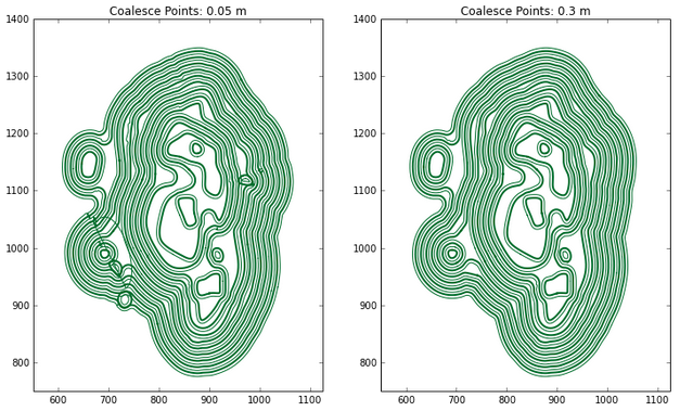
Figure 20: Left: possible geometry errors due to floating point precision and other edge cases. Right: After increasing merge points slightly, the errors are corrected.
Note: These are very sensitive parameters. Using too small of a number may lead to more errors, using too large of a number will significantly compromise the pit design (to the point that it will probably resemble an abstract piece of art more than a pit design).
If the units are in meters, and the pit covers a few dozen hectares suggested ranges for these parameters are tabulated below:
| Suggested Minimum | Suggested Maximum | |
|---|---|---|
| Filter Distance | 0.01 | 0.8 |
| Coalesce Distance | 0.01 | 0.5 |
These are certainly not set it stone, and some experimentation will be required. More complicated designs (many concave corners, multiple pit bottoms, etc.) may require different treatment.
Filter distance is measured perpendicular from a segment such that points within this tolerance are removed. This quantity is supplied in distance units. This can help to speed the calculation up, as well as remove troublesome points.
Merge points is measured between close together points such that they may be replaced by a new average point. This quantity is supplied in distance units. Note if errors arise after electing to constrain minimum mining width or the minimum outer radius, merge points is the primary weapon to remove them.
Midbench Cache
This parameter is only necessary when outputting midbench strings. This parameter controls the number of points in the midbench cache for any given set of toe / crest polygons. This is used internal to the algorithm and should generally be ignored. However, if the pit is very large and complicated (many concave corners) this cache might have to be increased. Using a very large cache may improve accuracy of the midbench strings, but will also greatly slow down saving the output.
Shard Area Cutoff
This parameter is only necessary when using block model input, and designing multiple phases at once. This parameter should be used in conjunction with the snap phases option in the input preprocessing tab.
On any given bench there may be several polygons from different phases which are very close together. These walls are shared between phases, and small deviations from that can lead to undesirable results. The polygon from the earlier phase may even extend outside the later phase, which would imply that some area should be mined in one phase and then filled back in in the subsequent phase. This is incorrect, so those parts of the inner polygon are removed. However there also may be small 'shards' that is pieces of a polygon along the boundary which are outside the earlier phase, but within the later phase. These shards should be removed. Any shard that has an area less than the given Shard Area Cutoff is included in the earlier phase.
This parameter is given in area units.
This section controls the format of the output which can then be used for future mine design. Design strings and/or triangulations may be generated based on the options in this panel.
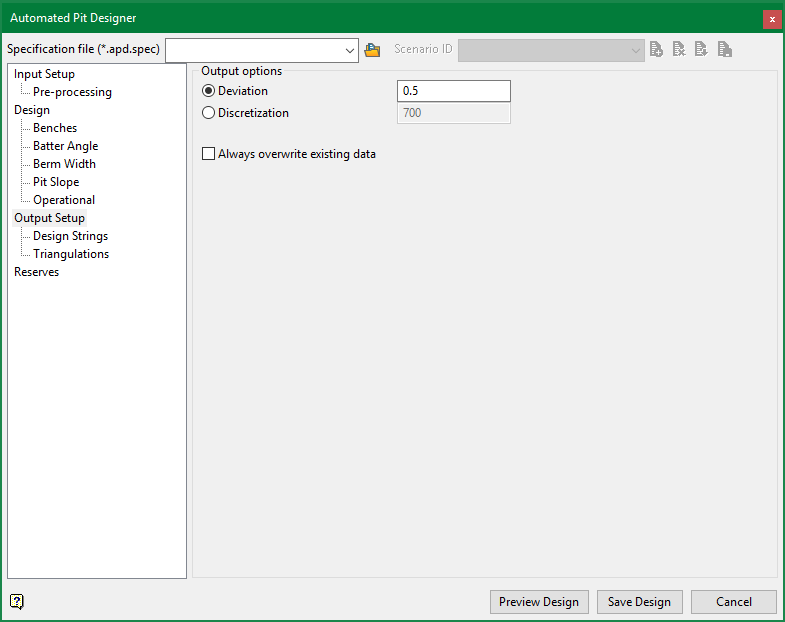
Output Options
Deviation
Specify the allowable deviation from the underlying curve. This directly controls the number of points / triangles in the result. The effect of the parameter is illustrated below.

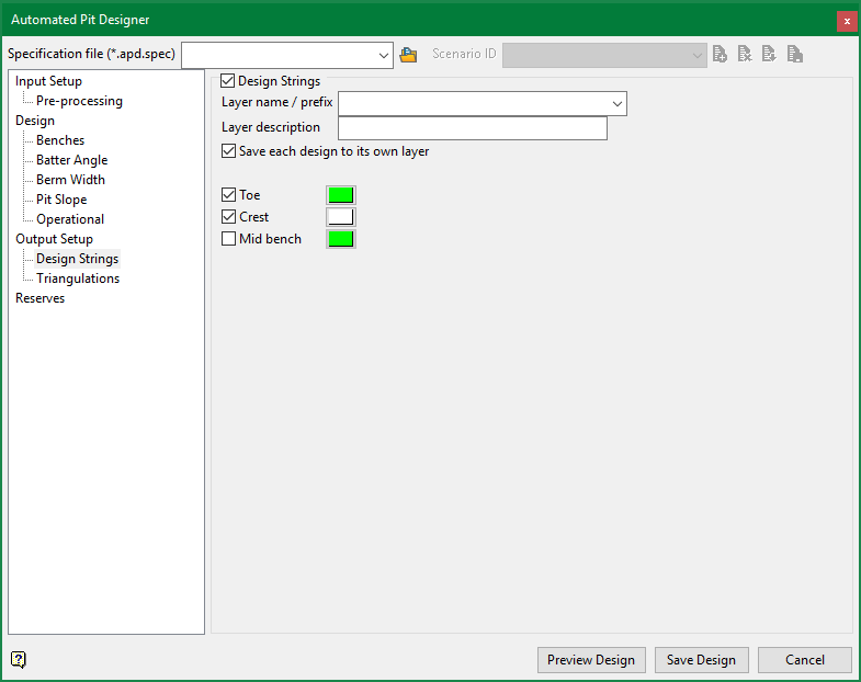
Design Strings
Layer name
Specify the layer name to save the resulting design strings into, if left blank the name will be inferred from the spec file / scenario.
Layer description
Specify the layer description.
Save each design to its own layer
Select this option to save each design to its own layer, this is only applicable if multiple phases are being designed from a block model. The Pit number will be appended to the layer name.
Design Strings
Toes, Crests, and/or Midbenches can be saved to the layer. Select the appropriate checkboxes and specify the string colour using the colour box.
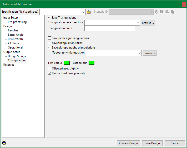
Triangulations
Triangulate save directory
Specify the directory to save the triangulations.
Triangulation Prefix
Specify a prefix for the triangulations, if left blank the triangulation name will be inferred from the spec file / scenario names.
Save pit design triangulations
Select this option if you wish to save the resulting pit design(s) as triangulations.
Save triangulation solids
Select this option if you wish to save the resulting pit design(s) as volumetric solids.
First Colour Last Colour
Specify the first and last colour to be applied to the triangulations. If the range is greater than the number of phases the colours will be evenly distributed between the first and last colour.
Offset Phases Slightly
If this parameter is specified the phases will be vertically offset from each other very slightly (on the order of 0.1 units) in order to remove the effect of 'z fighting' which comes from having many coincident triangles. This parameter should only be used for visualization. It should not be used when actually saving the design for further analysis.
Honor breaklines precisely
There are multiple methods to triangulate the toe and crest lines. Of the two currently implemented in the pit designer there are certain geometries where both are not ideal. Use this checkbox to switch between the two triangulation methods. When breaklines are honored precisely there should not be any flat triangles between toe and crest lines, this is generally appropriate, but with very complicated geometries it is not.
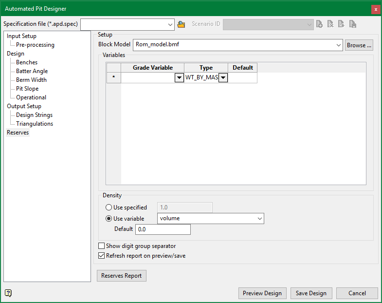
Setup
Block model
Select the block model that the reserve estimations will be based on.
Variables
Grade Variable
Select the grade variables from the drop-down list. There is no limit regarding how many grade variables can be specified for the calculation of reserves.
Type
|
Sum |
Used for variables containing units (for example, grams of gold) that should be cumulated rather than averaged. |
|
Wt by Vol |
Used for grade variables containing values based on volume weighted average (for example, grams of gold per cubic metre). |
|
Wt by Mass |
Used for grade variables that should be treated as a weighted average based on mass (for example, grams per tonne of gold). |
Default
Supply a Default value if you want to replace the construction default of the selected blocks during the reserve calculation. The construction default value is reported in a block model header.
Density
Use specified
Select this option to use a constant value when calculating the tonnage. You will need to specify the density value.
Use variable
Select this option to use the values contained in a specific block model variable when calculating the tonnage. The desired block model variable can either be entered manually or selected from the drop-down list.
Show digit group separator
Select this option if you wish to have the numbers formatted with comma separators. (Example: 1,000 instead of 1000.)
Reserves Report
Click this button to generate a report and view the results in a floating popup window.
Refresh report on preview/save
Select this option to generate a new report when Preview Design or Save Design are clicked. If this is not checked, a new popup window will not be generated when either of the two buttons are clicked. Note that a design that includes a lot of pits could take a long time to generate a report.

