Stereonet
The following table describes the tools in the Stereonet section of the Geotechnical tab.
| Tool | Description |
| Create Stereonet | Plots slope and slope direction (dip and strike) onto a two-dimensional graph. |
| Stereonet Contours | Creates stereonet contours. Stereonet contours are used to help identify discontinuity sets once a stereonet has been created. |
| Add Plane | Adds a plane to a stereonet. Adding a plane to a stereonet will result in a great circle being drawn and/or its pole. |
| Kinematic Analysis | Used to analyse discontinuity sets on a stereonet to determine likely failure mechanisms of pit face. |
| Blind Zone | Defines the region of trend and plunge of discontinuity poles that are perpendicular to those of drillholes used to take samples, should any exist. |
| Set Window | Used to draw a region on a stereonet encompassing certain trend and plunge spans. |
Create Stereonet
Before creating a stereonet, suitable data must be prepared. Note: If this data has previously been prepared and exported to .csv text file, it does not need to be recreated. The stereonet can be created from file data.
To prepare data:
-
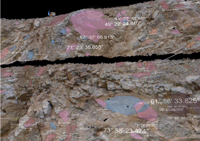
Select a triangulation created using spherical, scan triangulation or a fusion surface. Topographic triangulations are not suitable for geotechnical analysis as they are created in a top-down manner that does not provide sufficient detail on rock slopes.
-
Go to Geotechnical > Colour > Colour Dip and Strike to highlight the areas to be analysed.
-
Select point or facet selection mode.
-
Select some points on a structure of interest.
-
Go to Geotechnical > Dip and Strike > Extract.
-
Repeat this process (steps 2 - 5) for all structures of interest. Discontinuity objects are saved in the geotechnical container for each query.
To create a stereonet:
-
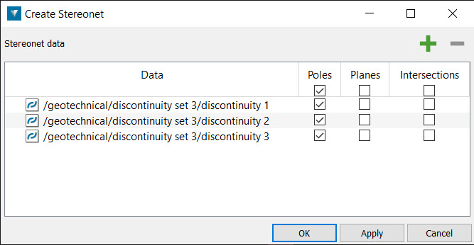
Go to Geotechnical > Stereonet > Create Stereonet. This will open a new panel.
-
Transfer discontinuity data to the Data field.
-
Select poles, planes or intersections.
-
Click OK or Apply to create a new stereonet in the geotechnical container.
-
Open the new stereonet in a view window. The stereonet toolbar will be displayed. Use the options available to set up the stereonet.
-
Select the Grid Style.
-
Select Scale poles if you want the poles to be sized according to their discontinuity/triangle area.
Here are some stereonet examples:
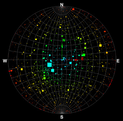
|
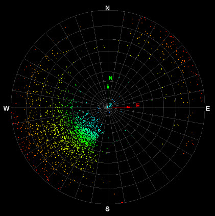 |
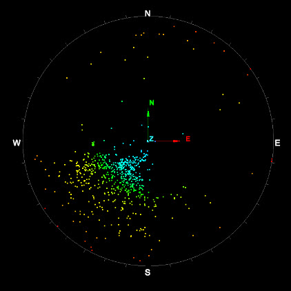
|
| Stereonet — Equal angle, Equatorial grid, Scale poles by area | Stereonet — Equal angle, Polar grid. | Stereonet — Equal angle, no grid. |
Stereonet Contours
Stereonet contours are used to help identify discontinuity sets once a stereonet has been created. The contours represent density distributions of poles and can be set as either wireframe or flat shaded regions. The user can adjust custom bandwidths of pole distribution and assign custom colours to these bandwidths. Smoothing and Terzaghi weighting are also options.
To create stereonet contours:
-
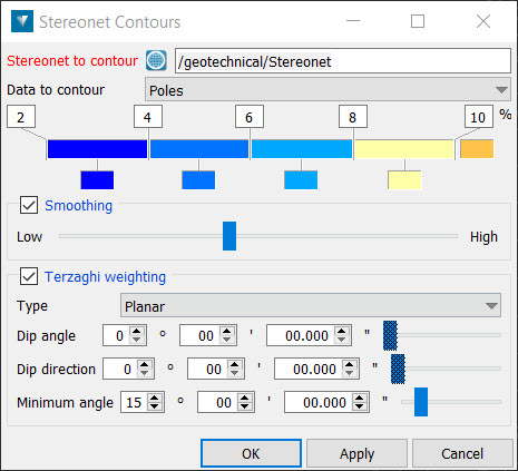
Go to Geotechnical > Stereonet > Stereonet Contours. This will open a new panel.
-
Drag and drop the stereonet into the Stereonet to contour field.
-
Select whether you want contours around poles or intersections. Select the colours and values for the percentage bandwidths to represent the data concentration.
-
Check Smoothing if required. If checked, adjust the slider accordingly to adjust the level of smoothing.
-
Check Terzaghi weighting if required. Terzaghi weighting uses the measurement orientation to counteract the sampling bias. If checked, set the Type (Planar or Linear), Dip angle, Dip direction and Minimum angle. The Minimum angle is the lowest angle between the measurement orientation and the discontinuity that will be used for weighting.
-
Click OK or Apply to generate contours. The contours are saved in the stereonet container.
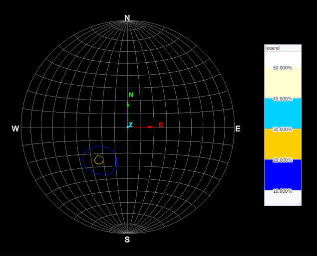
|
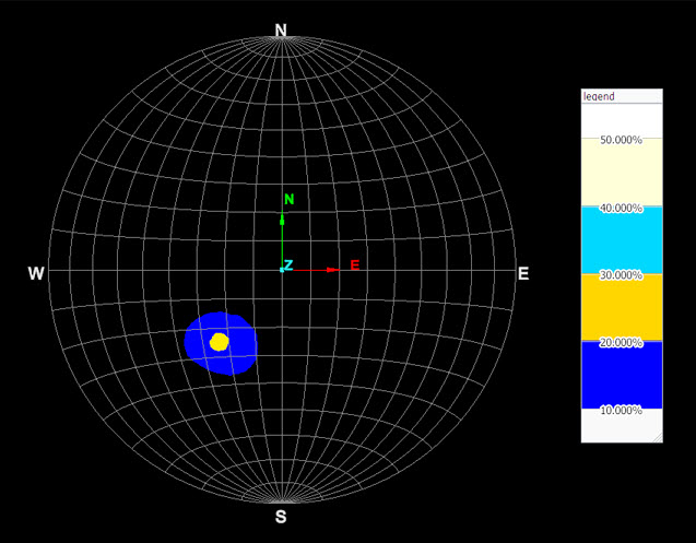
|
| Stereonet contour (wireframe) and legend. | Stereonet contour (solid) and legend. |
Add Plane
Adding a plane to a stereonet will result in a great circle being drawn and/or its pole.
Great circles can be used to visualise the orientation of the plane or joint set on a stereonet. A great circle can also be created from a cluster of projection poles and thus display an average plane for the cluster.
To add a plane:
-
Display the stereonet in a View window.
-
Display the fitted planes in a separate View window.
-
Go to Geotechnical > Stereonet > Add plane. This will open a new panel.

-
Using the facet selection tool, highlight the plane (or highlight a discontinuity object) to be used to create the great circle. The Dip angle and Dip direction are automatically populated. If more than one object is selected, the mean orientation is used.
-
Select whether to Display pole and/or Display plane. Select another colour if desired. Enter a location for the plane, if desired.
-
Click OK or Apply. The great circle is saved in the stereonet container specified in the Destination stereonet field.
Kinematic analysis
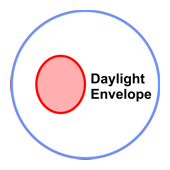
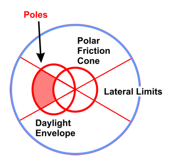
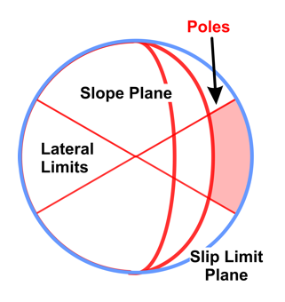
Kinematic analyses are conducted using stereonets on a collection of poles (normals of planes) and/or plane intersections selected from the discontinuities of a rock face. The analyses help to identify the kinematic feasibility for sliding, wedge and toppling failures in an excavated face. The components examined include slope dip, slope dip direction, daylight envelope, slip limit, lateral limits, polar friction cone and planar friction cone.
Use the Failure zone drop-down list to select the type of failure to be analysed. Fill in the appropriate values for the relevant criteria in the Kinematic analysis tool panel and examine the resulting stereonet to see if any poles and/or intersections are in critical zones. A kinematic analysis object will be saved into the stereonet container specified in the Destination stereonet field.
The following tables and diagrams will provide background information explaining the types of failures, critical zones and examples of relevant stereonet diagrams.
Note: You will need to ascertain likely friction angles and lateral limits appropriate to the rock faces and materials being investigated.
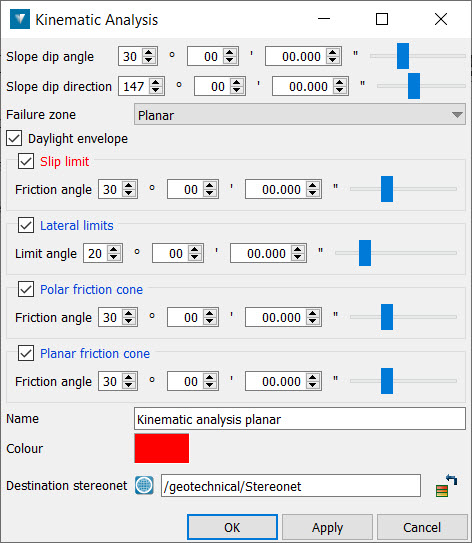
Here is the panel you will generate if you go to Geotechnical > Stereonet > Kinematic Analysis.
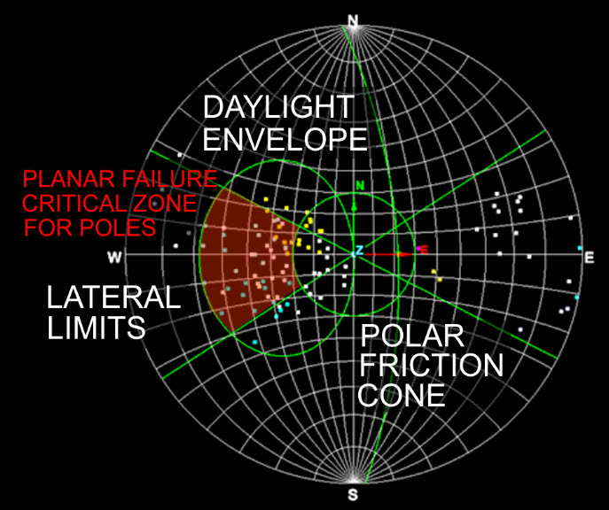
Here is a typical Kinematic analysis plot on a stereonet:
The Kinematic analysis components required for the analysis of each of the failure mechanisms is summarised in the table below.
|
KINEMATIC ANALYSIS COMPONENTS |
TYPICAL REPRESENTATION OF COMPONENTS ON STEREONETS |
FAILURE MECHANISMS |
|||
|
Note: Orientation and scale may be different according to actual planes under investigation. |
PLANAR |
WEDGE |
FLEXURAL |
DIRECT |
|
|
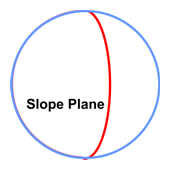
Slope dip Measured down from horizontal. |
Great circle plotted from the Slope dip and Slope dip direction of the pit wall, main rock face, etc. |
|
|
|
|
|
Slope dip direction Direction the slope runs directly
downwards.
|
|
|
|
|
|
|
Daylight envelope |
|
|
|
|
|
|
|
|
|
|
||
|
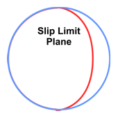
Slip limit
Greater circle representation of the plane at which friction slipping will occur. Poles (normals) closer to the outside perimeter of the main circle are steeper and will slide and/or topple.
|
|
|
|
|
|
|
Slip limit dip angle = pit slope angle - friction angle Slip limit dip direction = same as pit slope |
|||||
|
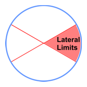
Lateral limits |
|
|
|
|
|
|
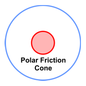
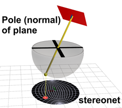
Polar friction cone |
|
|
|
|
|
|
defect plane dip > friction angle (assuming friction only) |
|||||
|
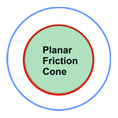
Planar friction cone |
|
|
|
|
|
|
line of intersection dip (between 2 discontinuities) > friction angle (assuming friction only) |
|||||
|
|
|
|
|
|
|
|
Poles (normals) |
|
|
|
|
|
|
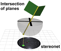
Intersections Point formed by the vector at the intersection of planes of interest (discontinuities). |
|
|
|
|
|

The following table displays the criticalstereonet regions and point types (poles and/or intersections) relevant to the analysis for the various failure mechanisms.
|
TYPE OF FAILURE |
CRITICAL REGION ON
STEREONET |
PROCEDURE |
|
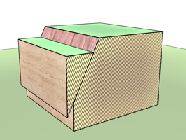
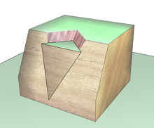
PLANAR FAILURE
Dislodgement and downwards sliding of blocks and/or layers along single common failure planes. |
|
Any critical poles occur outside the Polar friction cone, inside the Daylight envelope and between the Lateral limits.
|
|
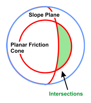
WEDGE FAILURE
Dislodgement and downwards sliding of blocks along two, intersecting, common failure planes. |
|
Any critical intersections occur inside the Planar friction cone and towards the outside (shallower) than the main slope plane.
|
|
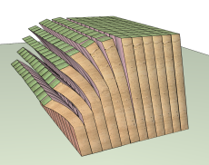
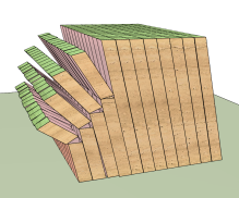
FLEXURAL TOPPLING
Forwards flexing and downwards sliding of steeply slanting blocks and/or layers. |
|
Any critical poles occur towards the outside of the Slip limit plane (steeper) and between the Lateral limits.
|
|
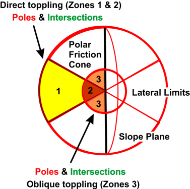
DIRECT TOPPLING
Breaking and toppling forwards of steeply slanting blocks and/or layers.
OBLIQUE TOPPLING As intersections approach vertical, toppling to the sides outside the lateral limits, becomes more likely. |
|
Critical Intersections - Zones 1 and 2 Indicator for Direct Toppling in conjunction with critical poles of Base planes (see below).
Critical Intersections - Zone 3 Indicator for Oblique Toppling in conjunction with critical poles of Base planes (see below).
Critical Poles of Base Planes - Zone 2 and 3 Base planes inside the Polar Friction Cone and therefore will not slide but still may provide a release mechanism to blocks.
Critical Poles of Base Planes - Zone 1 These Base planes may slip. Therefore, combined sliding and toppling modes may occur simultaneously.
|
Blind Zone
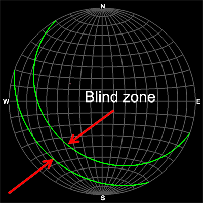
A Blind Zone on a Stereonet represents the region of trend and plunge of discontinuity poles that are perpendicular to those of drillholes used to take samples i.e. the discontinuities line up or are approximately parallel with the drillhole. This region is of interest because any potential discontinuities that line up with the drillhole are likely to be missed as they don't pass through (or intersect). Hence, there could be the possibility of many discontinuities around the drillhole but no samples in the drillhole.
Note: This tool defines a Stereonet region of an unknown quantity of discontinuities. There may be none, some or many.
Discontinuities missing the drill hole.
The region/band of trend and plunge representing a blind zone for a drillhole.
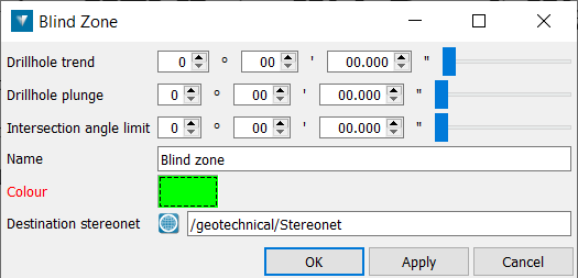
(Drillhole trend = 40° , Drillhole plunge = 60° , Intersection angle limit = 10° )
- Open the Stereonet intended to show the blind zone.
- Select Geotechnical > Stereonet > Blind Zone
- The Blind Zone panel will open - enter values into fields on panel.
- Select OK or Apply to create lines defining the Blind Zone limits on the Stereonet.
The inputs required:
- Drillhole trend — The angle from North (see Glossary).
- Drillhole plunge — The angle down from horizontal (see Glossary).
- Intersection angle limit — The extra angle around the Drillhole trend and plunge to create a band of similar values.
- Other information such as a Name, Colour (for the lines surrounding the zone) and Destination stereonet.
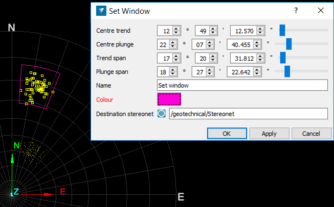
Set Window
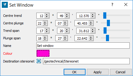
Set window allows the user to draw a window at a certain area on a stereonet.
The dimensions of the windowed area are defined by trend, plunge and spans around the trend and plunge. These figures can be entered manually.
Alternatively, selecting a group of poles can be used to auto-populate the window dimensions, or selecting a relevant Discontinuities container.
- Select Geotechnical > Stereonet > Set Window.
- Enter the Centre trend, Centre
plunge, Trend span
and Plunge span.
Alternatively, auto-populate trend, plunge and span values by selecting points (poles) on the stereonet, or selecting a Discontinuities container in the Explorer window. - Enter a Name for the window.
- Choose a Colour for the window frame.
- Choose a Destination stereonet to display the window.
- Click OK or Apply.
A stereonet with points (poles) selected and the resulting window drawn around them.