Tutorial - Ellipsoid Methods
The ellipsoid method allows you to dynamically enter several ellipsoids and then will interpolate between them. Averaging orientations is not easy. For example, the average of a bearing of 10 degrees plus a bearing of 350 degrees does not equal (350 + 10)/2, it is actually 0. To get around this, the tool uses a quaternion averaging method developed by NASA.
This tutorial requires the Aniso_tutorial dataset. Unzip the folder and save to a location from which you can open Vulcan. It will have all the files you need and should become your working folder during this tutorial.
Load the tutorial block model and display the model extents.
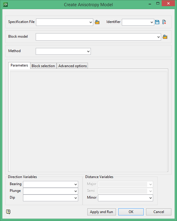
On the Block menu, point to Unfolding, then click Create Anisotropy Model to display the following panel.
Ellipsoid Method (Dynamically Entering Data)
The first way to use this tool is by dynamically entering ellipsoids.
Fill in the Create Anisotropy Model panel as follows:
Top Section:
Fill out a Specification file.
Fill out an Identifier.
Select block model = "tutorial.bmf".
Select the method = Ellipsoid.
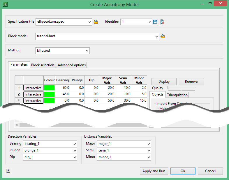
Parameter tab:
Click the interactive button select somewhere within the block extents and arbitrarily position the ellipsoid.
You can edit the parameter manually as well.
Add a second ellipsoid the same way.
Direction Variables:
Select bearing variable = bearing_1.
Select plunge variable = plunge_1.
Select dip variable = dip_1.
Distance Variables:
Select major variable = major_1.
Select semi variable = semi_1.
Select minor variable = minor_1.
Click  .
.
Because this is a persistent panel you can perform other operations while this panel is still up.
On the Block menu, point to Viewing, then click Load Dynamic Model to display the following panel.
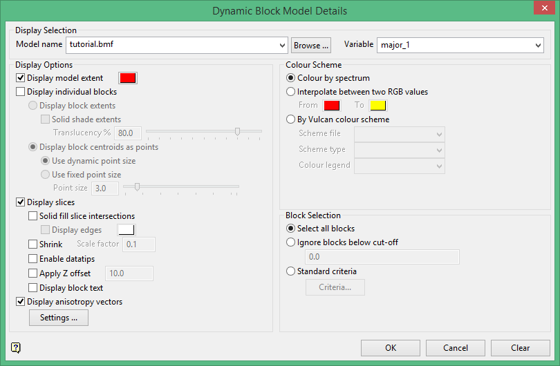
Display Selection
Model name = "tutorial.bmf"
Variable = "major_1"
Display Options
Display Model extent = yes
Display individual blocks = no
Display slices = yes
Solid fill intersections = no
Display anisotropy vectors = yes
Click 
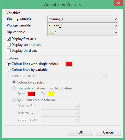
Bearing variable = bearing_1
plunge variable = plunge_1
dip variable = dip_1
Display first axis = yes
Colour Scheme
Colour by spectrum
Block Selection
Select all blocks
Click  to both,
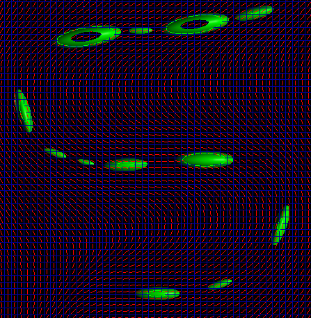
View the model in section view, plan view at 2m elevation.
You can see how the anisotropy vectors interpolate smoothly between the ellipsoids. Many more ellipsoids can be easily added to fine tune the results.
Because the Create Anisotropy Model is a persistent panel you can adopt the following very efficient workflow:
1. Modify / Add ellipsoids in the Create anisotropy grid.
2. Click apply and run, wait for the interpolation to finish, usually only a second or two.
3. Right click to access the context menu, reload dynamic model.
Ellipsoid Method (Design Data)
The second way to use the ellipsoid method is by importing the ellipsoids from design data.
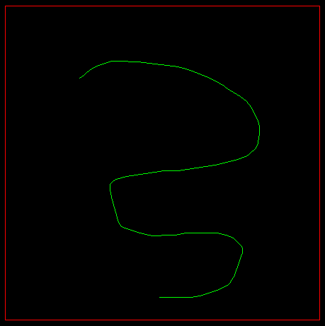
Load the block model extents.
Draw a squiggly line through the extents.
Next, create a new Anisotropy Model Identifier by typing a 2 into the textbox.
For this tutorial we will reuse the block model variables, so there is very little else to fill out.
Under the Parameters tab, delete the existing rows by selecting them, then right-click to bring up the context menu and select delete.
Instead of filling out the grid manually, use the Import from Objects panel on the right.
You can supply the Major, semi, minor axes - or set them based on the line segment.
You must supply a plane, this is generally just "Level". You cannot define an ellipsoid (considering dip) from a single line segment.
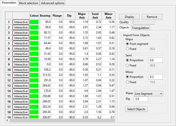
Select your squiggly line to populate the grid.
Select all of the ellipsoids in the grid, and click display (Note that the quality slider only applies to the displayed ellipsoids, nothing else).
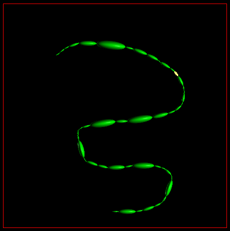
Click
Load up the dynamic model as before and note the vectors.
This can be much more efficient for rapidly entering ellipsoids than the manual method.
Variable method
The variable method uses the moment of inertia to ascertain bearing, plunge, and dip from an underlying continuous variable. For each block it uses a moving window to calculate an underlying covariance map for that region. It treats the covariances as weights and evaluates the moment of inertia. This allows it to estimate the underling direction of major continuity.
This method is very fragile, and often gives somewhat surprising result. We are investigating an improved method based on a multiscale principal component analysis, but that is not finished.
Create a new Block > Unfolding > Create Anisotropy Model Spec file and ID.
Fill out the panel, but select the Variable method.
Select the sim variable.
You can experiment with the window size. In the example, a window size of 5, 5, 3 was used (given that the model has 1m blocks).
Click
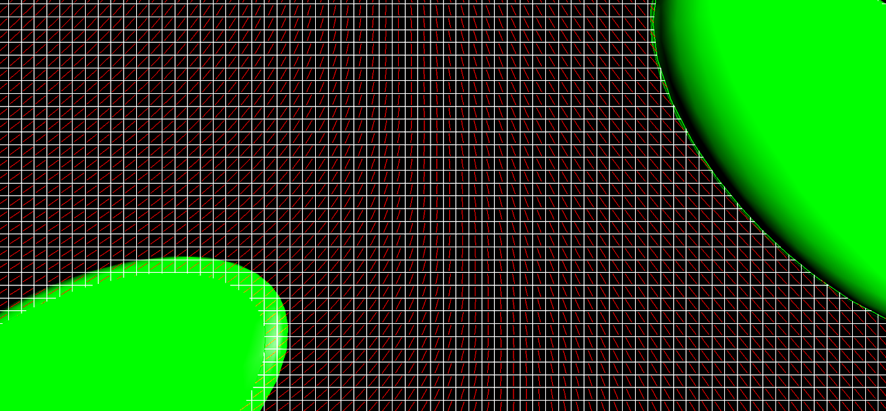
Load a dynamic model, only this time display the underlying sim variable as well.
Make sure your slice goes through the middle of the model with z = 6.
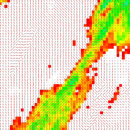
This upper left portion of the block model shows the vectors based on the variable sim.

