Model
Create Monitoring Data Models
Use the Model option to create models of the monitor data, that can then be used with the View > Animation option to provide 4D visualisation. The resulting model, may consist of triangulated surfaces, resulting vectors, grids, contours or point data. A model is generated for each time period (each sample location).Instructions
On the Open Pit menu, point to Monitoring, and then click Model.
Select a reference monitor.
Once selected, the following panel displays.
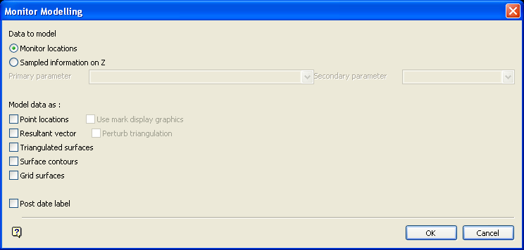
The selected reference monitor forms the time base against which the data extracted from all other monitors will be compared.
For example: If the reference monitor has samples at date 1-Jan, 2-Jan, 5-Jan and 7-Jan, then four models will be created. The data from the other monitors will be interpolated at those times.
If you need models at regular intervals, use the Display Settings option to set the time intervals so any monitor can be selected as the reference monitor.
Data to model
The model can be generated based on 3D location ( Monitor Locations ) or a 2D location with another parameter for the Z value ( Sampled information on Z ). The other parameter can be selected from the Primary parameters (that is, base and extra parameters) or from the Secondary parameters (parameters derived from the user definable fields).
For example, if you wanted to model the movement of a wall, then the prism locations alone would contain that information and you would select the Monitor locations field. If you wanted to create a model of the wall movement's absolute velocity (speed), then you would select the Sampled information on Z field with the Average Velocity as the Primary parameter.
Model data as
The modelling methods produce for each time period:
Point locations
A sample point is generated for each sample location from each monitor loaded. The locations are stored in a nominated layer. If you checked the Use mark display graphics check box, then the system will use the same symbols to create the point data. For example, if you display the sample points of the monitors using the diamond symbol, then when modelling, as points, you will get all the point data as diamonds.
Resultant vector
A vector is generated from the starting point of the monitor (reference point) to each sample location from each monitor loaded (this can be used to distort an existing triangulation). The vectors are stored in a nominated layer. The colour of the vectors will be taken from the same legend used for the vectors of the loaded monitors.
If you checked the Perturb Triangulation check box, then you will be asked to select a triangulation, typically a surface model, on which the monitors are located. The vectors are used to move the triangulation, simulating the movement of the surface.
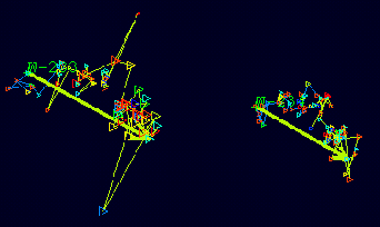
Diagram 1 - Original Monitor Data
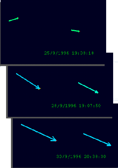
Diagram 2 - Modelled Points and Vectors from Animation Sequence
Triangulated surfaces
A triangulation is generated for each set of points. Each sample location, from each monitor loaded, at each recorded time, will form a triangulation. For example, if there are 20 recorded sample locations and 10 monitors loaded, then you will get 20 triangulations with 10 points in each.
Note Do not try to create a triangulated surface with only one monitor loaded.
Diagrams 3 to 5 show how displacement of the monitors, and hence the material, varies with time. You can see that on November 25 th (the red triangulation), the displacement of monitor W-233 was in the opposite direction than on the 25 th of October (the blue triangulation).
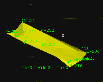
Diagram 3 - Triangulated Surface Representing Displacement at 25/9/1996 20:41:00 (yellow)
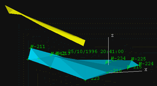
Diagram 4 - Triangulated Surface Representing Displacement at 25/10/1996 20:41:00 (blue)
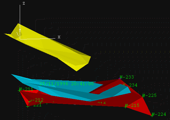
Diagram 5 - Triangulated Surface Representing Displacement at 25/11/1996 20:41:00 (red)
Surface contours
A set of contours is generated for each sample monitor locations, at each time recorded (similar to triangulated surfaces). This is useful in the visualisation of surface variation over time (use non-exaggerated point data). The process can be cancelled by pressing the [Esc] key.
Diagrams 6 to 9 show that on the 25 th of September, most of the movement/displacement was vertical and only at the top left edge of the area where the movement died out. In contrast, on the 25 th of October and in particular the 25 th of November, most of the movement occurred at the edges of the area, while the centre of the area did not experience significant movement.
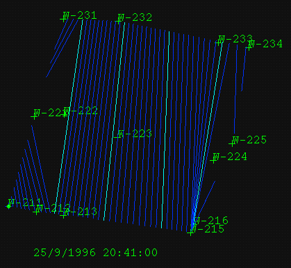
Diagram 6 - Contours Representing Displacement on 25/9/1996 at 20:41:00
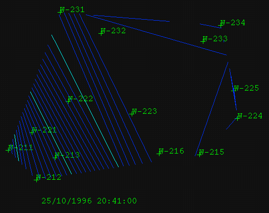
Diagram 7 - Contours Representing Displacement on 25/10/96 at 20:41:00
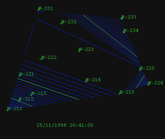
Diagram 8 - Contours Representing Displacement on 25/11/1996 at 20:41:00
Grid surfaces
A grid surface is generated from each set of sample monitor location points, at each recorded time.
Post date label
Select this check box to post the date (run time) as graphics. You will need to indicate the location to which the date is to be posted onto the screen, and its text parameters. We recommend that you do check this box, as it is very useful to know the date and time of each contour.
Note Performance of the system is proportional to the number of modelling methods enabled and the number of monitors loaded. We recommend that you don't enable more than two methods at the same time.
Click OK.
The panels and prompts displayed depend on the selected modelling method.
Point locations
Resultant vector
Triangulated surfaces
Surface contours
Grid surfaces
Point locations
The Point locations modelling method produces the following panel.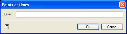
Layer
The maximum size of the layer name is 40 alphanumeric characters (spaces not allowed).
Click OK.
The point locations are then displayed on the screen.
Resultant vector
The Resultant vector modelling method produces the following panel.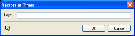
Layer
The maximum size of the layer name is 40 alphanumeric characters (spaces not allowed).
Perturbed model prefix
This refers to the triangulation file identifier (<tfi>) of the triangulation name. The full name will be <tfi>n.00t, where n = a number incremented for each generated triangulation. The total size of the prefix is 20 alphanumeric characters. This field is not displayed if the Perturb triangulation check box was not selected.
Click OK.
If more than one triangulation is loaded, then you will be asked to select which triangulation to perturb. Otherwise, the loaded triangulation is selected.
Triangulations for each vector will then be created. A vector is created from the starting point of the monitor (the reference point), to each individual sample point, that is, if a monitor consists of 200 sample points recorded, you will get 200 vectors and triangulations.
Once the modelling has been completed the vectors displays on the screen.
Triangulated surfaces
The Triangulated surfaces modelling method produces the following panel.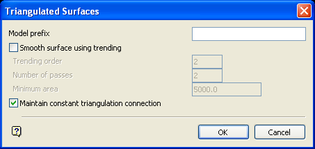
Model prefix
This refers to prefix part of the file name of the triangulations to be created. The full name is <prefix>n.00t
,
where n = a number incremented for each generated triangulation. The total size is 20 alphanumeric characters, including the file extension.
Smooth surface using trending
Select this check box to build a trend into your model. The trend represents a best fit mathematical model that estimates the surface shape between the data points.
The mathematical method used is a regression method that gives the best fit. In the same manner that you can plot a scatter diagram and work out a line of best fit, you can add an extra variable (For example, easting or northing) and compute a 3D surface of best fit. The fitted surface represents the regional trend present in the data. This trend surface will pass through the data as a surface of best fit. The data necessary to apply trending is specified through a separate panel. This panel is accessed upon completion of the current panel.
Only applicable when the Smooth surface using trending check box is enabled.
Trending order
It relates to the complexity of the trend surface. See the table below for an indication of the order to use.
| Order | Surface |
|---|---|
| 1 | Plane surface |
| 2 | Dome or simple syncline (paraboloid) |
| 3 | Folded surface (anticline and syncline) |
Number of passes
Only applicable when the Smooth surface using trending check box is enabled.
It specifies the number of smoothing passes to be applied to the triangulation once it has been created. Smoothing applies a mathematical equation that calculates the variance of the modelled data. Once the value has not changed from the previous calculated variance by a certain percentage, the iterations or calculation process discontinues. Nine smoothing passes are usually sufficient.
Minimum area
Only applicable when the Smooth surface using trending check box is enabled.
It to specify the minimum area to be smoothed.
Maintain constant triangulation connection
Select this check box to maintain a constant topology for each triangulation. The topology is the way in which each vertex is connected, via edges, to its neighbours. The triangulation is created independently for each time, and it is possible that as monitors move, the topology could change. For example, an edge is created at one time, where there was no edge in the previous time as the monitor points have moved closer together. Checking this box preserves the topology from the first time, and uses it in all subsequent times. Not maintaining the topology means other properties derived from the triangulation, such as contours, will experience dramatic changes as a result of topological differences.
Surface contours
The Surface contours modelling method produces the following panel.
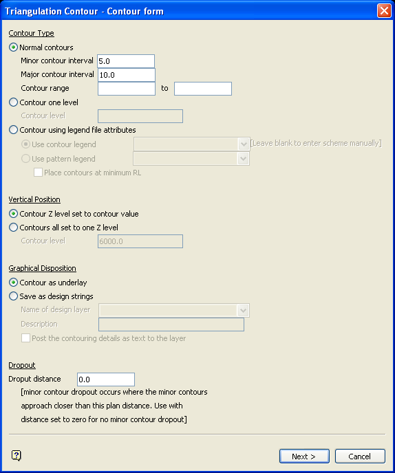
This panel to specify the type of contours. Refer to the Model > Contouring > Contour option for more information on this panel.
Select Next.
The following panel is then displayed.
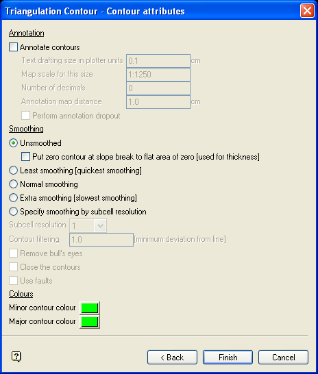
This to specify contour colours, whether smoothing is required, and to annotate the contours. Refer to the Model > Contouring > Contour option for more information on this panel.
To generate the contours, the option creates its own internal triangulation that is not kept. By default, it keeps the constant triangulation connection, that is constant topology .
Grid surfaces
The Grid surfaces modelling method produces the following panel.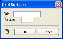
Grid Surfaces panel
Grid
This refers to the grid model identifier (<.gfi>) of the model to be created. The maximum size is 10 alphanumeric characters, spaces are not allowed.
The full name is <proj><gfi>/<mv>g, where <proj> = project, <gfi> = grid model identifier, <mv> = model variable and "g" denotes a grid mesh (compared to "t" for triangulations).
Variable
This refers to the model variable (<mv>) part of the grid file name extension.
Click OK.
The following panel is then displayed.
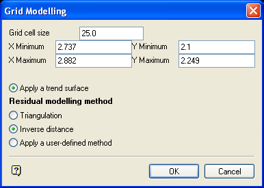
Apply a trend surface
Select this option to apply a trend surface.
Residual modelling method
The available methods are Triangulation, Inverse distance and user-defined. Refer to the Grid Calc > Model > Grid Model option for details on these methods. The panels displayed below show the panels that you can expect with each method.
The Triangulation method produces the following panel.
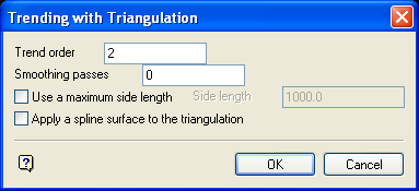
Trend order
See Trending order above.
Smoothing passes
See Number of passes above.
Use a maximum side length
Select this check box to set the maximum length for a triangle side. The data mask will be set to zero for grid points in the triangulations that have a side.
Apply a spline surface to the triangulation
Select this check box to produce grids from smoothed triangulation data. Breaklines are recognised.
The Inverse Distance method produces the following panel.
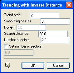
Trend order
See Trending order above.
Smoothing passes
See Number of passes above.
Power
This refers to the inverse distance power. The default value is '
2
'.
Search distance
Specify the maximum search radius for the inverse distance method. The data mask will be set to zero for grid points that were evaluated using points further than this distance from the grid point. The default value is unlimited search distance.
Number of points
Specify the number of interpolative points to be used by the inverse distance method. The default value is '10'.
Set number of sectors
Select this check box to set the number of sectors. This to divide the search area into sectors, so that data selected for modelling does not come from a cluster of points. The maximum number of sectors allowed is 8.
The User Defined method produces the following panel.
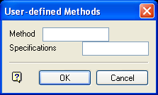
Method
This to access any customised modelling methods previously set up using the Grid Calc > Edit Modelling Defaults > Define Method option.
Specifications
Enter the Grid Calc specification file (file extension.gdc_spec). The specification file is created through the Grid Calc > Edit Modelling Defaults > Create Grid Specifications option.
This option allows for the modelling of data displayed on the screen and/or the data that exists in the prisms database. It is possible to model the resulting vectors, display contours, create triangulations for each time period etc.
Click OK.
Once all the appropriate panels have been completed, the gridding process commences. A message window is displayed to inform you of the date and time currently being modelled. The process can be stopped by pressing the [Esc] key.

