Editing & Modelling an Orthogonal Variogram
After the experimental variograms have been calculated you can model them using these controls.
Properties tabs
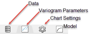
Data Tab
There are no special functions under the Orthogonal Variogram Data Tab.
Variogram Parameters Tab
Variogram Mode
Refresh Chart
To refresh the chart, click the ![]() icon in the upper right corner.
icon in the upper right corner.
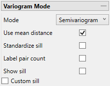
Mode
(Click to expand)
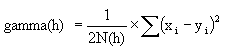
Semivariogram
This is the standard semi variogram.
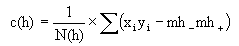
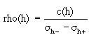
Covariance
Correlogram
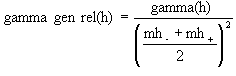
General relative semivariogram
This is like the standard semi variogram, but divided by the mean of the data values.
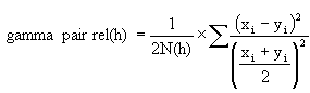
Pairwise relative semivariogram
This is like the standard semi variogram, but each difference is divided by the mean of the sample values.
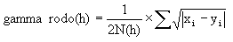
Rodogram
Madogram
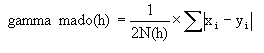
Madogram Ratio
sqrt(Semivariogram) / Madogram
Use mean distance
Use the mean distance for the x coordinate of the variogram points.
Standardise sill
Select this check box if you want to standardise the variogram sill by dividing the results by the sample variance. This is useful when calculating a semivariogram because instead of reaching the sill at the sample variance it will reach it at 1.
Label pair count
Select this option to display the number of pairs used for each point on the graph.
Rotate pair count
This option displays when Label pair count is selected. Select this option to rotate the number labels of the pairs so that they are oriented 90 degrees upward.
Minimum pair count
Enter the lowest number of pairs that you want to be used to influence the variogram model.
Show sill
Select this option to show the sill.
Custom Sill
Select this option to enter your own value for the sill.
Direction Settings
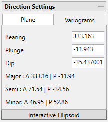
Figure 1: A = Azimuth; P = Plunge
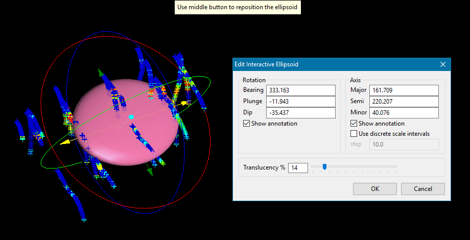
Interactive Ellipsoid
Click this button to open an interactive window in the Vulcan 3D viewer. You can use the controls on the ellipsoid to set the direction parameters.
Data Analyser allows you to input the plane orientation and from there obtain the three variogram directions. This can be done before or after the chart has been created. The input plane is the same used in the model for that variable.
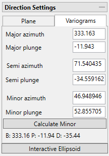
The angles for Major, Semi-major, and Minor are automatically calculated from the settings entered in the Plane tab, however, you can edit those settings if you desire. If the Semi-major is not orthogonal (90 degrees) to the Major, then a warning will be given. However, it is not required that the angles be orthogonal to each other. If you want the minor angle to be orthogonal to the Major and Semi-major, then click the Calculate Minor button and the two angles will be automatically filled in.
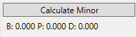
Click the Calculate Minor button to perform the calculation. The results will provide the bearing, plunge and dip based on the Major Azimuth.
Down Hole
It is common practice to calculate a down hole variogram to acquire a nugget, and then use that nugget value while calculating a standard variogram.
Omni-Directional
An omni-directional variogram considers all directions in the same calculation. It can be thought of as an average variogram of multiple directional variograms. However, it doesn't mean that the spatial continuity is equal in every direction.
Omni-directional variograms are a good starting point when trying to look for the structure of the overall continuity of a domain.
Major, Semi-major and minor Settings
Directional Properties
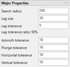
Search radius
The search radius should correspond to approximately half the distance of your data field. if the search radius is greater than the halfway point, then the search will over-extend the edge of the data.
If the distance traversing your sample area is 500 feet, then set the search radius to 250 feet.
Lag size
The lag size is the distance for each step from the origin. Set a lag size that coincides with your data spacing.
If your samples are spaced 50 feet apart, then set your lag size to 50. If you have to err, do so on the side of too small.
Lag tolerance
The lag tolerance is the distance plus or minus the lag size that samples will be captured. This helps capture samples that are not located at the exact distance interval as the lag spacing. Set the distance within which to use samples.
Note: If this is set to 0, then the tolerance is not used.
Samples are rarely located at exact intervals such as every 50 feet throughout the entire domain. There will nearly always be some variance. You can capture the samples that are not at exact intervals by setting the variogram to recognise samples that fall within 25 feet of the lag size, which in our sample case is every 50 feet.
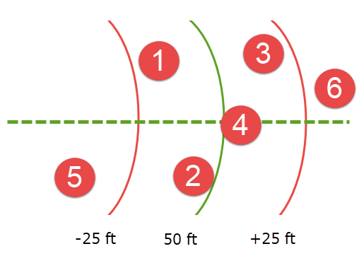
Here, the green line represents a lag size of 50 feet, and the red lines represent a lag tolerance of 25 feet on either side. Samples 1, 2, 3, and 4 would be used in the calculation. However, samples 5 and 6 would be ignored.
Lag tolerance ratio
This corresponds to the percentage of the lag size that is used by the lag tolerance.
A lag size of 50 with a lag tolerance of 25 will result in a lag tolerance ratio of 50%.
Azimuth
Enter the azimuth. This parameter controls the azimuth direction in which variography is evaluated.
Plunge
Enter the plunge. This parameter controls the plunge direction in which variography is evaluated.
Tolerance thresholds
Collectively, the azimuth tolerance, plunge tolerance, horizontal tolerance, and vertical tolerance are known as the Cone of Tolerance. Using too large of a cone can result in excessive mixing of samples from different directions. This can cause the apparent anisotropy to appear smaller than the true anisotropy. Using too small a cone can result in rough variograms that are hard to interpret. The sample cone may be too small if the number of sample pairs for most lags is small compared to the number of sample points.
For an omnidirectional variogram, use 90 for the azimuth tolerance and 90 for the cone angle tolerance.
Note: At a great enough distance, the horizontal distance tolerance and vertical distance tolerance will clip the sides of the search cone.
Azimuth tolerance
Enter the limit on the angle between two samples as measured in the plane of the plunge of the variogram.
Plunge tolerance
Enter the limit on the angle between two samples as measured in a vertical plane in the direction of the azimuth.
Note: A combination of cone, azimuth and plunge tolerances is used if the azimuth angle tolerance and plunge angle tolerance are set to less than the cone angle tolerance.
Horizontal tolerance
Enter the horizontal distance limit on sample pairs. Any acceptable sample must be within this horizontal distance of the centre of the variogram cone.
Tip: Set this value to a typical spacing (or larger) between your data, for example, if your data is on a 100 × 100 × 10 grid, set a horizontal distance of 100 and a vertical tolerance of 10. If you receive too few sample pairs, try increasing the tolerances to capture more data otherwise artifacts such as "hole effects" may occur.
Vertical tolerance
Enter the vertical distance limit on sample pairs. Any acceptable sample must be within this vertical distance from the centre of the variogram cone. The vertical distance is measured from the plane of the plunge of the variogram cone.
Copying parameters from one direction to another
You can copy the parameters from one direction to another by right-clicking on the heading bar of the source and selecting Copy or Copy parameters to all directions, or Paste but keep direction.
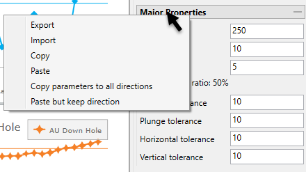
If you click Copy, then right-click on the heading bar of the properties you want to paste the contents to, then select Paste.
If you click Copy parameters to all directions, the content is automatically pasted to the other directions.
Similarly, if you select Paste but keep direction, the content is automatically pasted to the other settings but the direction is maintained.
Backtransform Normal Score
![]()
This option simulates the back transformation of the current variogram into the real variable, which is usually easier to model.
View Cones in Vulcan
You can visualise the search ellipses by enabling the option to View Cones in Vulcan, or by clicking Display Cones from the Connectivity tab in the ribbon. The cones are interactive, therefore, any changes made in the variogram parameters will be automatically reflected in the cones seen in Vulcan.

Steps
-
Begin by clicking the button labelled Pick in Vulcan.
-
In the Envisage workspace, click where you want the origin of the cones to be displayed.
-
Use the slider to adjust the Translucency of the cones.
-
Set the colours for the cone by clicking on Colour 1 and Colour 2, then selecting a colour from the palette.
-
To remove a the cone from the screen, disable the View Cones in Vulcan checkbox.
After you have set the parameters for a cone, it can be displayed using the icons found on the Connectivity tab on the ribbon.
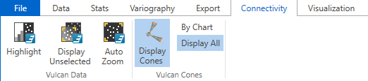
Click Display Cones, then select either By Chart or Display All.
By Chart - Only the charts that have the View Cones in Vulcan option enabled will be displayed.
Display All - All cones will be displayed regardless of whether or not the View Cones in Vulcan option has been enabled.
Create Deferred Scattered
Each variogram point is the average of a collection of points that have a distance (h) from the origin point. Therefore, each variogram point can generate a correlation between the origin point and the others inside the indicated neighbourhood.
First, select a point from the variogram.
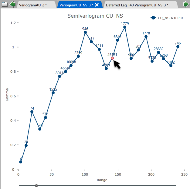
Next, click the Create Deferred Scatter button to create the chart.
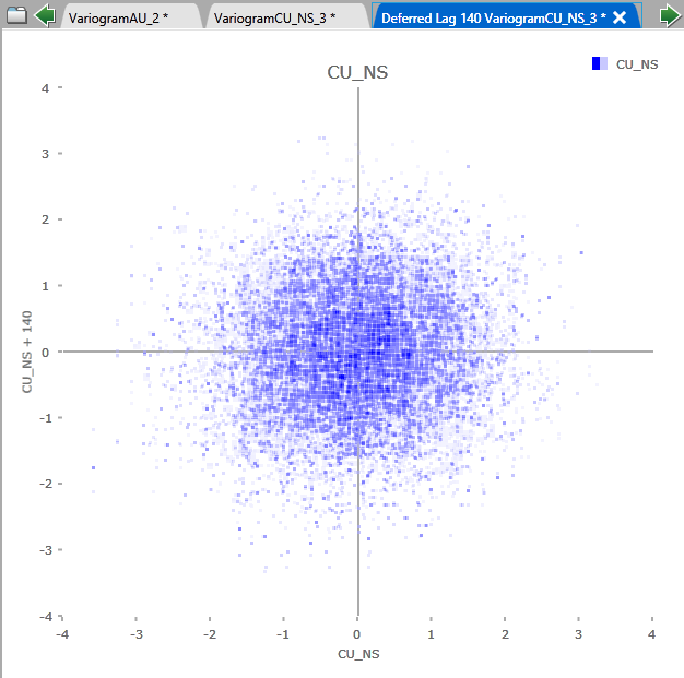
Chart Settings Tab
Chart Area
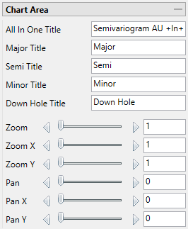
Here you can customise the titles of the charts.
Chart Display Options
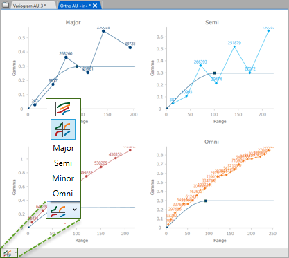
In the lower left corner of the chart window, use the drop-down list to select how you want to display the charts in the window.
Options include:
-
All models in one chart.
-
All charts in grid view.
-
Each chart separately.
Data
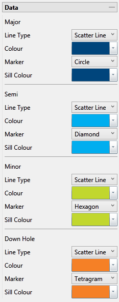
Colours and Markers
Use the drop-down menus to select the colours and markers to customise the charts.
Axes Settings
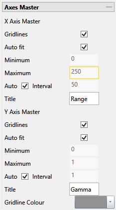
Gridlines
Select this option to display the gridlines at major intervals on the chart. You can elect to display gridlines for both axes or just one, depending on your needs.
Auto fit
By default, Vulcan Data Analyser will auto fit the axes based on the values calculated from the dataset. However, you can customise the axes to highlight your particular study and needs. This can be done in two ways:
Method One
-
Deselect Auto fit.
-
Set a Minimum and Maximum range.
-
Let Vulcan Data Analyser adjust the intervals automatically by leaving the Auto Interval option selected.
Method Two
-
Deselect Auto fit.
-
Set a Minimum and Maximum range.
-
Deselect Auto Interval, then enter an interval of your choice.
Axes Titles
By default, the axes are provided with the traditional titles of Gamma and Range. However, if you wish to change these you may do so by replacing the text in each of the textboxes.
Gridline Colour
Click the arrow to display the colour palette, then select a colour for the gridlines.
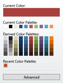
Clicking the Advanced button will bring up a dialog which will allow you to customise the colour to you exact specifications.
All in One Models
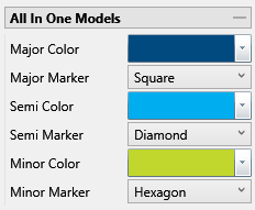
Use these controls to edit the models Major, Semi-major, and minor colour and markers.
Note: This will only work when the chart is set to display all the models in one chart.
Annotations and legend
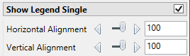
Horizontal and Vertical Alignment
Click and drag the legend in the chart to the desired position or enter a number to position the chart legend.
Show Legend Single
Use this option if only one chart is showing in the chart area. See Chart Display Options above.
Show Legend Multi
Use this option is you have multiple charts showing in the chart area. See Chart Display Options above.
Model Tab
Model
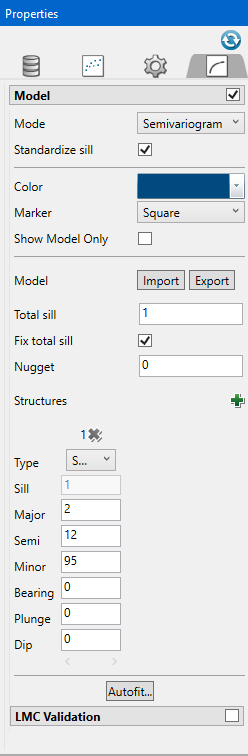
Mode
Semivariogram
This is the standard semi variogram.
Covariance
Correlogram
General relative semivariogram
This is like the standard semi variogram, but divided by the mean of the data values.
Pairwise relative semivariogram
This is like the standard semi variogram, but each difference is divided by the mean of the sample values.
Rodogram
Madogram
Madogram Ratio
sqrt(Semivariogram) / Madogram
Standardize sill
Select this check box if you want to standardise the variogram sill by dividing the results by the sample variance. This is useful when calculating a semivariogram because instead of reaching the sill at the sample variance it will reach it at 1.
Colour and Marker
Use the drop-down menus to select the colours and markers to customise the charts.
Show Model Only
Select this option to display only the line representing the model in the chart. The individual points will not be displayed.
Model Import / Export
A model can be imported in or exported out. The files are stored as <filename>.vrg. The models that are exported out can be used in block model estimations.
Total Sill
If you do not know the exact sill, enter a number that is close. Start with a whole number or a number rounded to 0.5 and work from there. The sill you choose will not affect the model calculations. It will only affect how you are able to see it on the chart.
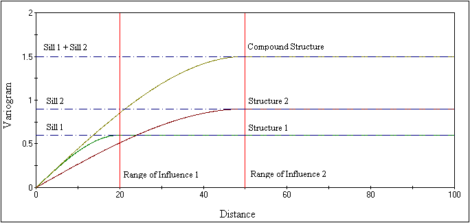
The total sill is equal to the nugget plus all the structures such that
Total Sill = Nugget + Structure 1 + Structure 2 +... + Structure n
Fix total sill
Enabling this option prevents the sill from being changed when setting up the structure(s).
Nugget
You can enter the nugget obtained from the down hole variogram or enter another nugget. The default nugget is 0.
The nugget is the variance at an infinitely small separation distance.
Structures
Additional structures can be added by clicking the green ![]() icon.
icon.

When the green ![]() is clicked, a context menu will appear. The menu will show the types of structures available.
is clicked, a context menu will appear. The menu will show the types of structures available.
![]()
|
General |
This option will be used most of the time. Use this if the experimental variogram has a standard look. |
|
Zonal Anisotropic |
Use the Zonal option when the range of the experimental variogram is extremely long. Typically, the variogram may never reach the sill. With this option, the search distance of at least one direction must be set. |
|
Cyclic Anisotropic |
User the Cyclic option when the experimental variogram looks like a sine wave as it approaches the sill. Only two types of structures are available when this option is selected: Periodic and Hole Effect. With this option, the search distances for two of the three directions must be set to a maximum distance of 999999. |
|
Isotropic |
This option is similar to the General option. However, all search distances will be the same for each direction. |
Type
Define the type of structure by choosing from the drop-down list.
In some instances, a variogram cannot be characterised by one of the model variograms described previously. However, a combination of models may adequately represent such behaviour. The final variogram structure is therefore termed a nested structure. Spherical models are often nested, with each component model reflecting a particular scale of variability in the deposit. Modelling of nested structures is generally by trial-and-error.
Search Distances & Orientation
Enter the search distances into the Major, Semi-major and minor textboxes. Then enter the orientations into the Bearing, Plunge and Dip. You can see the affect altering the orientation of the search parameters will have on the model by adjusting the sliders.
Autofit
Click the Autofit button to open the Autofit panel. The progress bar  in the lower left corner will show you the progress. You can also hover your mouse over the Autofit button to see how many iterations have been calculated and the error between one iteration and the next. You do not need to wait until the autofit function completes. You can stop it at any time. The model will be drawn in real time on the chart and you will be able to see the changes as the autofit function calculates through the iterations.

