Herco Analysis
Use this option to generate grade tonne curves for a given block size. You can use affine, indirect log-normal correction, and discrete Gaussian model as the support change engines. The analysis can be performed using multiple variables and using multiple cutoffs.
To use the Herco Analysis tool, you will need:
- A samples or composite database.
- A free output field if the change of support is requested to be stored in the samples database.
- A block model (optional). The block model is used as a reference when used to validate block model estimations.
Instructions
On the Block menu, point to Grade Estimation, and then click Herco Analysis.
Follow these steps:
-
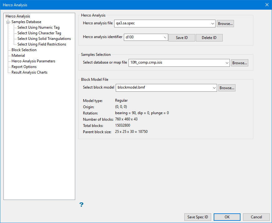
Select a specification file or enter a new name for the specification file in the space labelled Herco Analysis File. Click Browse to search for a file in a location other than your current working directory.
-
Select a Herco Analysis identifier, or enter a new ID and click Save ID.
-
Select a samples database or map file.
-
Select a block model (optional). The Model Type, Origin, Rotation, Number of blocks, Total blocks, and Parent block size will be automatically populated if a Vulcan block model is selected.
Samples Database
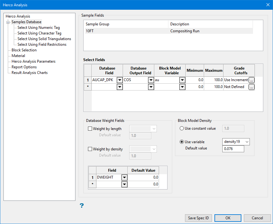
Here, select the groups to analyse and the variables. For each variable selected, a new tab is created on the Herco Analysis Parameters tab. Weighting is allowed for both samples (for example, length or decluster) and block model (density). Output support corrected data in the samples database is also possible.
Specify a table group identifier. Wildcards are supported. Only data from matching sample groups are selected. Press Ctrl while clicking on the group names to add/remove a group to/from the selection. Right-click to select all groups in the database.
Follow these steps:
-
Select the sample group from the database which will be analysed.
-
Select the fields using the table.
-
Database field - The samples database field that will be analysed for different support sizes.
-
Database output field (optional) - Select a field where the support-transformed grades will be written. If no field is selected, the transformation will not be written to the database.
-
Block Model Variable - Ideally, this is the same variable as the database field. This field is used to represent the output in mass unit and to validate the results. If this variable is not defined, the output is represented as a percentage or proportion of the total mass.
-
Minimum - This is the minimum value that is used to filter the input data for the database and block model fields. The value of the database field and the block model field must be between the minimum and maximum.
-
Maximum - This is the maximum value that is used to filter the input data for the database and block model field. The value of the database field and the block model field must be between the minimum and maximum.
-
Grade Cutoffs - Grade cutoff values may be specified as a range (first and last values), increment, or explicitly by value. Click
 to display the panel and set the values.
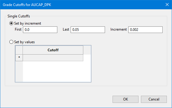
-
-
Select any database weight fields you want to use. Use this option for a database field only. For support change, select the weighting that will be used to calibrate the support values to a valid measurement. By default, the weight is one. There is no need to define a database weight if you do not use weighting fields.
-
Weight by length - If the database has a defined drill length, this is used as weighting.
-
Weight by density - If the database has a defined drill density, this is used as a weighting.
-
-
Define other weighting values using the drop-down list in the table, and enter a default value for each.
-
Select the Block Model Density if a block model field is being used.
-
Use constant value - Use this option to select a constant for defining the weight and default value.
-
Use variable - Use this option to select density variables for the calculation of reserves. Enter density variables manually or select them from the drop-down list.
-
Select Using Numeric Tag
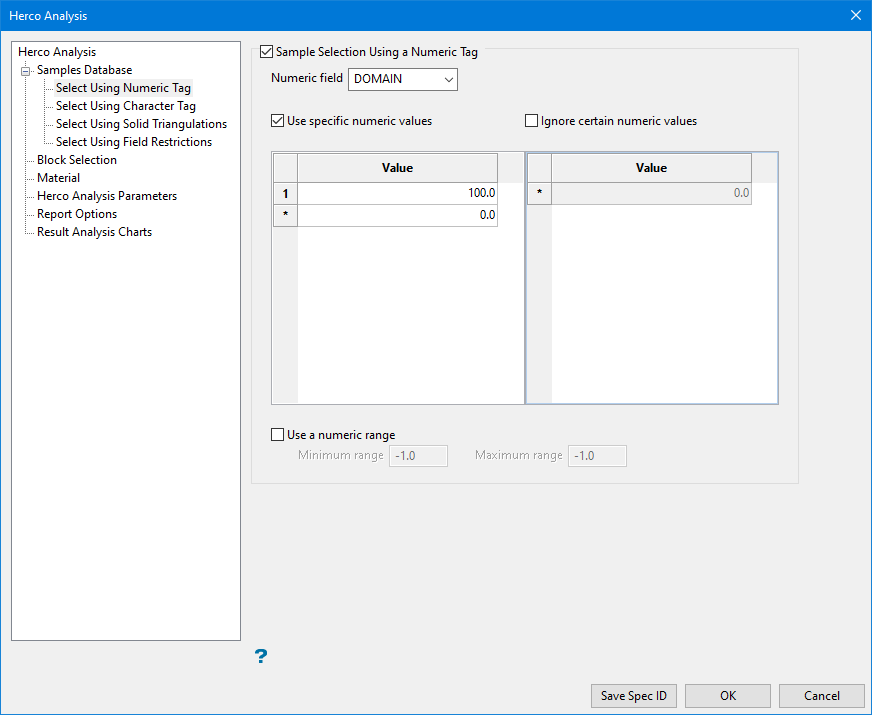
Use this tab to limit the samples to a specific numeric field. Once you select the numeric field you want to use, you can select specific values to use or ignore.
Follow these steps:
-
Click Sample Selection Using a Numeric tag to activate the filter.
-
Select the variable to filter by using the Numeric field drop-down list, then set the parameters that will determine how those values are treated.
-
Use specific numeric values - Only the values listed here will be evaluated.
-
Ignore certain numeric values - Any values listed will be ignored.
-
Use a numeric range - Use this to allow all value between a minimum and maximum number to be used.
0 to -9999 to ignore all negative values.
Note: The selection methods accumulate, that is, if more than one method is chosen, then the samples must satisfy each selected method before being included. Within a method, however, selection is based on the OR selection criterion except for field restrictions, which allows AND/OR selection criteria.
-
Select Using Character Tag
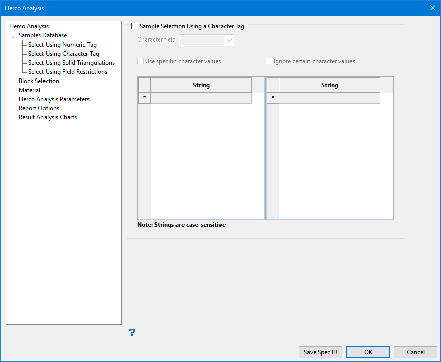
Select this checkbox to limit the samples using a specific character field. Once you select the character field you want to use, you can select specific character strings to use or ignore.
Follow these steps:
-
Click Sample Selection Using a Character tag to activate the filter.
-
Select the variable to filter by using the Character field drop-down list, then set the parameters that will determine how those values are treated.
Example: You may have a database field named MATERIAL and the entries in this field are 'ore', 'waste', and 'internal waste'.
-
Use specific character values - Only the values listed here will be evaluated.
-
Ignore certain character values - Any values listed will be ignored.
Note: The selection methods accumulate, that is, if more than one method is chosen, then the samples must satisfy each selected method before being included. Within a method, however, selection is based on the OR selection criterion except for field restrictions, which allows AND/OR selection criteria.
-
Select Using Solid Triangulations
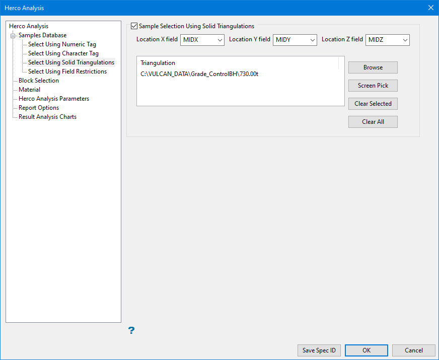
If you use this option, only the samples that fall in the boundaries of selected triangulations will be included. You will need to select this checkbox in order to add the necessary triangulations.
Follow these steps:
-
Click Sample Selection Using Solid Triangulations to activate the filter.
-
Select the X, Y, and Z coordinate fields for the dataset.
-
Select the triangulations you want use.
Browse button- The Triangulation Selection panel will be displayed.
 Triangulation Selection panel
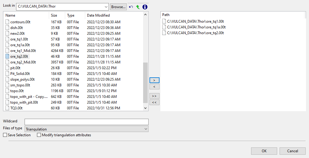
File Selection
Browse for files using the Browse... button, or use the interface showing the available grid files in the current working directory.
Click on the name of the file(s) you want to select. Use the
 icons to go to the last folder visited, go up one level, or change the way details are viewed in the window.
To highlight multiple files that are adjacent to each other in the list, hold down the Shift key and click the first and last file names in that section of the list.
To highlight multiple non-adjacent files, hold down the Ctrl key while you click the file names.
Move the items to the selection list on the right side of the panel.
- Click the
 button to move the highlighted items to the selection list on the right.
 - Click the
 button to remove the highlighted items from the selection list on the right.
 - Click the
 button to move all items to the selection list on the right.
 - Click the
 button to remove all items from the selection list on the right.
Wildcard
Enter the text to use as a filter, then press ENTER.
Use an * for multiple characters or a % to replace a single character.
Save Selection
Select this checkbox to save the selection list (the right-hand side of the Open panel), in a nominated selection file (
.sel). Once this panel has been completed, the Save As panel displays.Select the file that will be used to store the triangulation selection list. To create a new file, enter the file name and file extension.
Modify triangulation attributes
Select this checkbox to modify the current display attributes for the selected triangulation files. This option is recommend if you don't want to use the display settings from a previous Vulcan session. Once this panel has been completed, the Triangulation panel displays. Altering a triangulation's display attributes updates the modification date stamp (date modified).
The Modify triangulation attributes checkbox is not applicable to triangulation files that are currently loaded on screen. Use the Attributes option (under the Model > Triangle Utility submenu) to modify a loaded triangulation's display attributes.
Click OK to return to the main panel.
Screen Pick button- Allows you to select a triangulation that is currently loaded on the screen.
Clear Selected button - Removes all selected triangulations from the list.
Clear All button - Removes all triangulations from the list.
- Click the
Select Using Field Restrictions
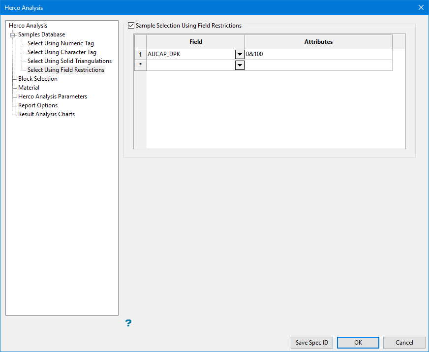
Select this checkbox to limit the samples to those with fields that match certain selection criteria.
Follow these steps:
-
Click Sample Selection Using Field Restrictions to activate the filter.
-
Select the Field for which the attribute conditions must be applied from the drop-down list.
-
Enter the conditions that must be true for the samples to be included into the Attributes column.
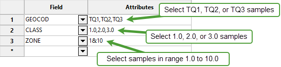
Include spaces in the entries in the Attributes column only if spaces are included in the desired field values.
When entering a range, always enter the smallest number specified before the largest number.
-792&-720since-792is smaller than-720. This range is evaluated as-792.0 ≤ VALUE < -720.0.A list of available operators/functions is provided in Appendix B of the Appendices > Core Appendices documentation.
Block Selection
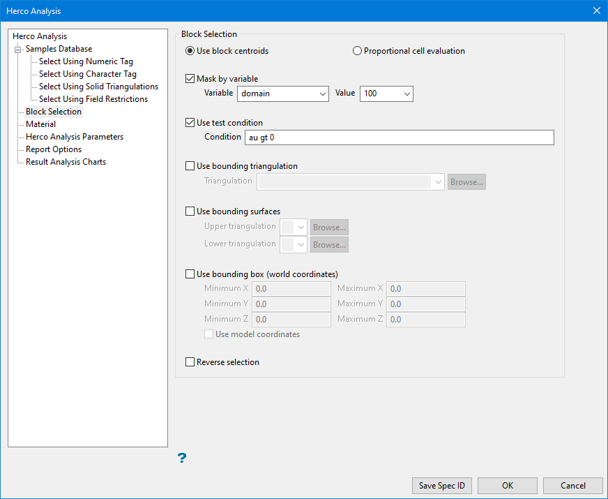
Use this panel to specify which blocks should be included in the analysis.
-
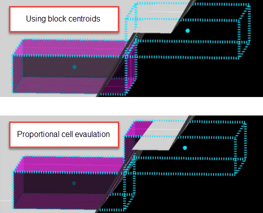
Decide whether you want to use the entire block in the calculations or only the portion that is within the regional boundaries. By default, the evaluation method is set to Use block centroids; however, you can select between Proportional cell evaluation and Use block centroids. This is especially important when using options such as Bounding triangulation, Bounding box, Section thickness, or Bounding surfaces.
-
Set the criteria for which blocks will be used by selecting one or more of the following options:
Important: Block selection is cumulative. Therefore, all arguments defined on this panel must be satisfied for a block to be included.
You will need to specify the variable, as well as a particular value.
If you have a variable called
Materialin your block model and want to restrict blocks to those where the material equals ore, selectMaterialas the variable and enteroreas the value. However, if you require all blocks that do not have this specified value, then enable the Reverse selection checkbox towards the bottom of the panel.You can also limit the blocks by Use test condition for a numeric block model variable.
To select blocks where iron has a value greater than 10.0, the condition would be
Fe GT 10.0The maximum size of the condition is 256 alphanumeric characters. Refer to Appendix B of the Core Appendices for a full list of available operators and functions.
This is useful when you want to evaluate reserves in a particular solid triangulation, such as a stope.
Select the triangulation from the drop-down list, or click Browse to open the Explorer to select a triangulation that is not in the current working directory.
Select the Upper triangulation and Lower triangulation from the drop-down lists, or click Browse to select triangulations from a location other than your current working directory. Only blocks that lie in the overlapping sections of the surfaces, as viewed in plan view, are selected.
If you select this option, you must enter the minimum and maximum coordinates for X, Y, and Z in the block model coordinates (X, Y, Z CENTRE). If the block model origin is set at 0,0,0, then real world coordinates should be entered in the X, Y, and Z minimum and maximum coordinates. If the block model origin is set at real world coordinates, then enter coordinates for the bounding box that are offset a certain distance from the origin. The distance of offset will be determined by the dimensions of your bounding box. It will be the distance to the minimum and the distance to the maximum X, Y, and Z from the origin of the block model.
Select the Reverse selection checkbox if you want to exclude the selected blocks within the slice. If this checkbox is not selected, the entire block is included within the slice by default.
Material
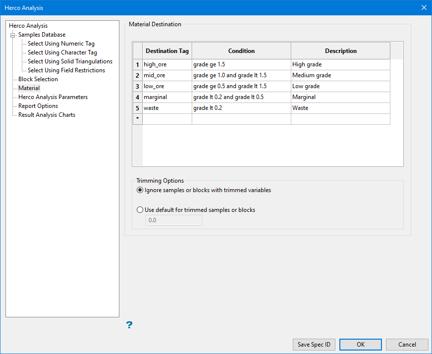
Use this panel to define the conditions to classify and identify the products and materials in the selected samples.
If a block model has been selected, variables for both the block model and the database need to have the same name since the conditions will be applied to both.
Follow these steps:
-
Enter an ID name for the material (short name) into the Destination tag column.
-
Enter the Condition that will be applied to the samples and block model data. If the variables are not selected in the Samples Database tab, the validation of these conditions will not be performed. Refer to Appendix B of the Core Appendices for a full list of available operators and functions.
-
Enter a Description of the material or product.
-
Select whether to Ignore samples or blocks with trimmed variables or to Use default for trimmed samples or blocks.
Herco Analysis Parameters
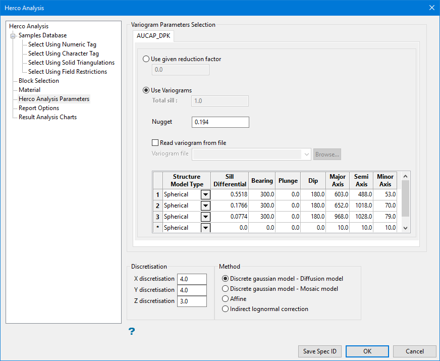
On this panel, you will select the variogram model, discretisation, and method (Affine, DGM, ILC). The tabs appearing across the top of the Herco Analysis Parameters panel are determined by the variables selected on the Samples Database branch. For each variable selected, a new tab will be created on the Herco Analysis Parameters tab.
Follow these steps:
-
Select between Use given reduction factor or Use a variogram.
Use given reduction factor
Enter a reduction factor between 0 and 1. The reduction factor is commonly defined as the ratio of block variance to sample variance. A factor close to one suggests the two variances are similar either due to a highly selective SMU size or geologic continuity; little mixing of material will occur (Rossi & Deutsch, 2013). A small factor value indicates the opposite and there will be a significant change in variance and resources above cutoff, at the selected SMU scale (Harding & Deutsch, 2019).
The reduction factor can be calculated from the variogram average. (Use the Variogram Average option to calculate the average of a variogram value.) The resulting output, which display through the Report Window, can be used to calculate the variance reduction factor for indicator methods, such as Indicator Kriging and Indicator Simulation, and also as an aid to defining the cell size for the block model used in Sequential Gaussian Simulation. The result may also be used in volume-variance correction and change of support models.
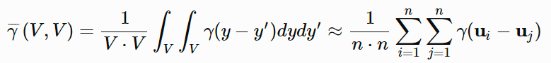
Figure 1: Average Variogram
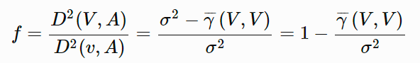
Figure 2: Variance Correction Factor (reduction)
Use Variograms
-
Enter the sill.
-
Enter the nugget. This represents the random variability and is the value of the variogram at distance (h) ~ 0.
-
Select Read variogram from a file to use an existing variogram model.
-
Select the Structure Model Type to be used from the drop-down list in the table. The variogram model type can be one of the following:
-
Spherical - This type is the most commonly used for ore deposits. They exhibit linear behaviour at and near the origin then rise rapidly and gradually curve off.
-
Exponential - This type is associated with an infinite range of influence.
The sill is reached at the sill range. In release 3.2 and earlier you had to enter a sill range of 3 times the actual sill range. To use this model, enter the effective range of the sill. For backward compatibility, see the exponential model 3. -
Gaussian - This type exhibits parabolic behaviour at the origin and, like the spherical model, rises rapidly. The Gaussian type reaches its sill smoothly, which is different from the spherical model, which reaches the sill with a definite break. The Gaussian model is rarely used in mineral deposits of any kind. It is used most often for values that exhibit high continuity.
-
In release 3.2 and earlier, you had to enter a sill range of 3 times the actual sill range. To use this model, enter the effective range of the sill. For backward compatibility, see the Gaussian model 3 below.
-
Linear - This type is a straight line with a slope angle defining the degree of continuity.
-
De-Wijsian - This type is a representation of a linear semi-variogram versus its logarithmic distance.
-
Power - This type is computed as M - d**p where M = the maximum correlation defined as 1000.0, d = distance from the origin, p = model power. For this model type only the power p is the major axis radius. Adjust the size of the ellipsoid so that the major axis is the desired power. The size of the ellipsoid for this model does not change the calculation of the variogram.
-
Exponential Model 3 - This is an un-normalised exponential model for compatibility with release 3.2 and earlier. The input radius must be the effective radius multiplied by 3.
-
Periodic - This is a sine wave with one complete period over the effective range. This model is not commonly used because it can cause samples at greater distances to have higher correlation.
-
Gaussian Model 3 - This is an un-normalised Gaussian model for compatibility with release 3.2 and earlier. The input radius must be the effective radius multiplied by 3.
-
Dampened Hole Effect - Dampening is achieved by multiplying the covariance function by an exponential covariance, that acts as a dampening function.
-
-
Enter the Sill Differential. This represents the difference between the value of the variogram where it levels off and the nugget.
-
If you have a total sill of 1.0, and a nugget of 0.15, you want your sill differential to be 0.85 = (1.0 - 0.15).
-
Enter the bearing (rotation about the Z axis), plunge (rotation about the Y axis), and dip (rotation about the X axis) of the variogram.
-
Enter the radii of the major, semi-major, and minor axes of the variogram.
-
-
Enter the Discretisation that is used for calculating the gammabar.
-
Select the Method that is used for analysing the support change. The method could be discrete Gaussian using either the diffusion or mosaic model, affine, or indirect log-normal correction.
Note: Explanations and diagrams of the different models are taken from the paper Flexible Change of Support Model Suitable for a Wide Range of Mineralization Styles, D.F. Machuca-Mory, O. Babak and C.V. Deutsch.
Discrete Gaussian - Diffusion model
Use this method when there are variables that exhibits a gradual spatial change, with high values separated from low values, but with a continuous spatial transition between them.
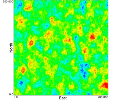
Figure 3: Diffusion type variable.
Discrete Gaussian - Mosaic model
Use this method for deposits showing a high continuity (or even identity of values) within a region or partition followed by abrupt changes in the transition from one partition to another.
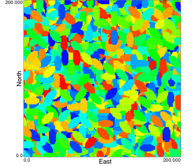
Figure 4: Mosaic type variable.
Affine
Affine variance correction is an approach to modify Z values to have lesser variability -- that is, to account for a larger-volume support. The affine correction leaves the shape of the histogram unchanged and shifts data values closer to the mean, depending on the magnitude of variance reduction.
 Indirect Lognormal Correction
A modified version of the log-normal correction designed to adjust the change in the mean that results when applying the log-normal correction to a distribution that is not a log-normal distribution. The correction is done by rescaling the quantiles
 of a log-normal correction by the ratio or the original mean,
  , over the mean
  of the values after the log-normal correction

where
is a quantile of the new distribution obtained by applying the indirect log-normal correction.Note: In addition to rescaling, the indirect log-normal correction lowers the skewness and increases the symmetry of the distribution. (Geostatistical Glossary and Multilingual Dictionary)
Report
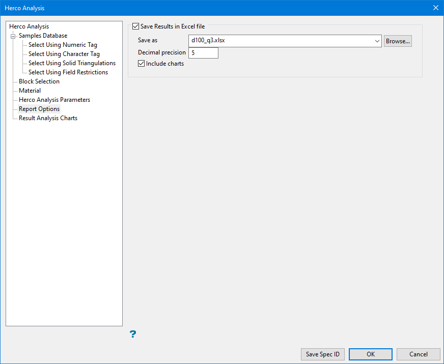
Use the Report tab to save the results of the Herco Analysis into an Excel File. The results are saved into sheets, and each sheet has descriptive name based on the file name and the type of process performed, such as single, multiple, or material.
Follow these steps:
-
Select Save Results to Excel file to output the result to a spreadsheet.
-
Enter the name for the Excel report.
-
Define the desired precision of the decimal.
-
Select this checkbox to create charts in the Excel report.
Results Analysis Chart
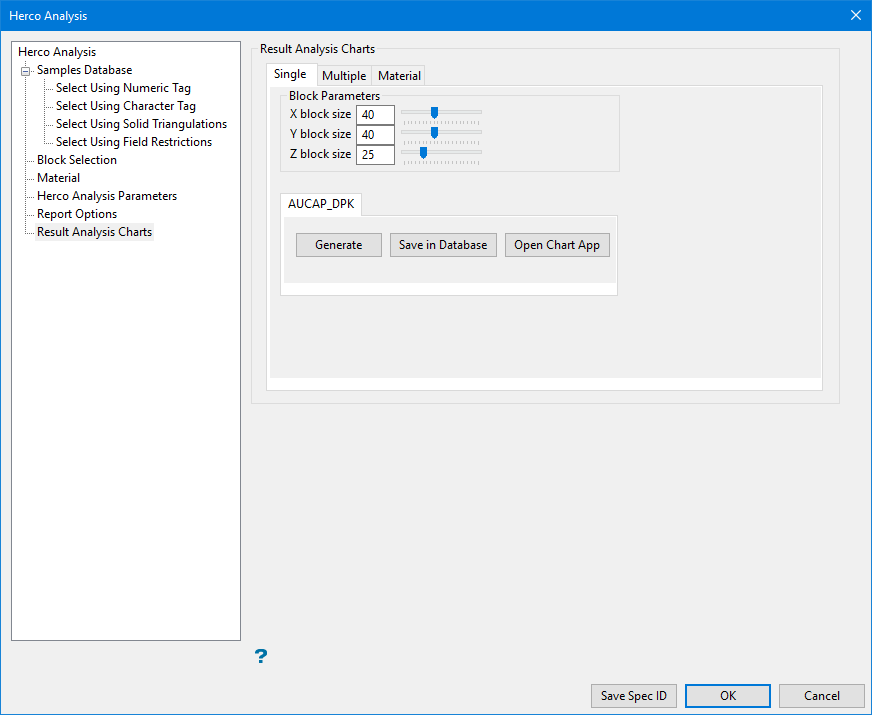
Use this panel to select Single, Multiple, or Material options for the charts.
Single
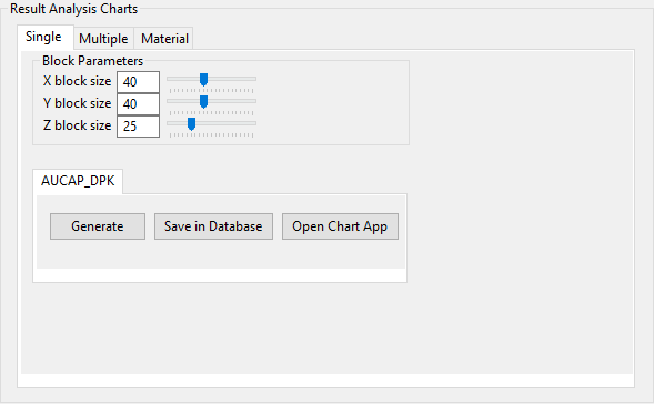
A single block size is analysed.
Enter the block size parameters and click Refresh to process the blocks geometry with the given variable. The output is a grade tonne chart for the variable, using the weightings, the correcting factor that is calculated from the variogram average, and the block size.
You can only save the results in the database if the Output field is defined in the Samples Database branch. You can also view the chart and manipulate it as desired, such as adding a watermark, viewing labels, zooming, scrolling, or saving it as an image.
Note: The Save in Database field will only be enabled if an entry has been provided in the Database Output Field on the Samples Database branch for the selected variable.
Multiple
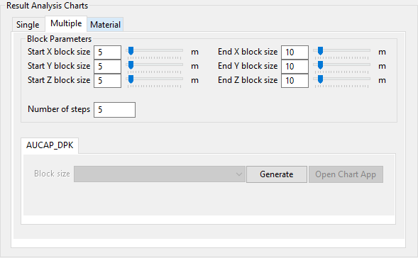
Multiple block sizes are analysed. The start, end, and steps for multiple block sizes must be entered. The output is a group of grade tonne charts. Each chart has a cutoff that represents the limit by which the chart is placed. This cutoff list is the one defined in the Samples Database branch. If the cutoff is changed, the chart displays for each one.
Material
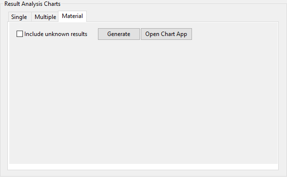
Material conditions are evaluated to generate a representation of mass and grade. The output is a bar chart representing the materials and the mass accumulated for each one. If block model fields are defined, the mass is represented in the unit of the block model. Otherwise, it uses the proportion of the total mass. You can also view the chart in 2D and 3D and manipulate it as desired, such as adding a watermark, viewing labels, zooming, scrolling, or saving it as an image.

