Modelling
The Modelling group of the Analysis ribbon contains tools that calculate and predict different blast performance indicators of a tie-up.
You can select the desired tie-up in the data explorer or view window. Each tool will automatically recognise the tie-up’s source data and perform the analysis based on this data. The only exception is the Fly Rock Modelling tool (see Fly Rock Modelling) which requires you to select the blast and data source you wish to use. An advantage of this is you can apply the modelling tools to snapshot data by creating a tie-up with a snapshot data source. For more information on snapshots, see Snapshot.
Each modelling tool will also recognise if the tie-up you select contains reconciled charge and times. The tie-up will contain these actual initiation times and reconciled charge, if you have selected the Use reconciled charge and times radio button in the tie-up editor. For more information on this option, see Using reconciled charge and times.
 Observation History
The Observation History tool displays a panel of the history of vibration observations for a site.
To use the observation history tool, follow these steps:
-
On the Analysis ribbon, in the Modelling group, select
Observation History. The Observation History panel appears.
-
To filter the data presented in this table there are four options which can be applied using the Filter button. Any number of these filters can be applied to the table and clicking Filter when all filters are unchecked will cause all observations to be displayed.
-
Filter by monitoring station: One or more monitoring stations can be selected from the drop-down menu and only observations from those stations will be displayed.
-
Filter by tag: Entering text in the Tag field will filter the list to only contain observations that have a tag containing the entered text.
-
Filter by detonation location: This will display all observations with detonation coordinates within the specified Filter radius of the location provided.
-
Filter by date: Only observations which were recorded between the first and last dates provided will be shown.
-
-
To enter data, click the Add entry button. This will open a new panel.
In the new panel, the following needs to be noted:
-
In the Monitoring section, select a monitoring station from the drop-down menu. This list is the list of locations for this site as defined in File > Setup > Site > Locations.
-
At least one of either PPV or Overpressure must be defined.
-
In the Blast section, there are two methods of entering an observation result: From tie-up or manual entry. Using the From tie-up option requires a valid tie-up object to be middle-mouse dragged from the explorer to the tie-up field. BlastLogic will then calculate the Detonation coordinates, MIC and Detonation time from this tie-up using a Timing window and Propagation rate provided by the user. The detonation coordinates are defined as the collar location of the closest hole to the monitoring station which contributed to the MIC.
-
An optional tag may be entered to help identify this vibration observation.
-
Click OK to save the vibration observation and close the panel.
-
-
Delete row will remove a selected observation from the table. This also removes the vibration observation from the BlastLogic server database.
-
Import from CSV will load vibration observations from a CSV file.
-
Export table to CSV saves the currently filtered vibration observations in the table to a CSV file.
-
The vibration observation table can be edited by double-clicking an editable cell and any changes made will be saved by clicking Save changes.
 Vibration Modelling
Vibration modelling aims to predict the ground movement caused by blasting. It is measured in either mm/s or inches/s and aims to calculate the peak particle velocity (PPV) of a blast at a specific location. This is the largest vibration within a timing window which is usually set at 8ms.
To open the Vibration Modelling panel, go to Analysis > Vibration > ![]() Vibration Modelling.
Vibration Modelling.
Model parameters
Vibration is dependent on explosive mass and explosive timing. BlastLogic enables the user to enter the following inputs:
- Propagation rate — the speed at which vibrations propagate through rock.
- Timing window — the time frame within which the Maximum Instantaneous Charge (MIC) is calculated.
- Extent — the distance to evaluate from the blast. Larger extents will require longer calculation times.
Calculation of PPV
Peak particle velocity (PPV) at a particular location in BlastLogic, is calculated using the following procedure:
-
Collect and order each detonation event within the timing window.
-
Calculate the total explosive mass and minimum distance to the point of interest at each detonation event.
-
Calculate the particle velocity for each total explosive mass and minimum distance to the point of interest using the following (referenced in the Australian Standards (AS) 2187.2, 2006):
 , where the site variable and site exponent are constants set in Setup > Site > Location.
 -
Find the maximum value for every timing window interval to obtain the PPV.
Background model information
In the basic case scenario (one hole with a single primer), the Maximum Instantaneous Charge (MIC) is calculated from the explosive mass loaded in the hole and the vibration for each point on the grid is calculated using the square root scaled distance formula. When there are multiple holes (or multiple explosive decks in a hole), the first primer to detonate in each explosive deck is used to calculate the initiation time and the mass entire explosive deck is used as the MIC. Secondary primers in explosive decks are ignored.
For each point in the grid, the propagation rate and initiation time per explosive deck are then used to determine which decks are interacting with each other by taking in consideration the time for vibration wave to reach the point (i.e. distance / propagation rate) and a provided timing window.
The charge mass is therefore calculated to be the sum of all charge masses of all the decks whose vibration waves reach the same grid point within the timing window. The MIC is calculated as the maximum of these charge mass sums. This is then used in the square root scaled distance formula to calculate the vibration at the given point.
Important: As the initiation time of a primer is required to determine the interaction of the vibration waves originating from different explosive decks, any hole that is not part of a tie-up will be ignored by the blast modelling tools. Additionally, holes that have no charge plan will have no effect on the model as they have no charge mass. If a hole has no primers but has been included in the evaluated tie-up, the entire hole is counted as a single explosive deck and the initiation time used is the initiation time of the hole.
Where?
To open the Vibration Modelling panel, go to the Blast Modelling drop-down menu and select Vibration.
Panel overview
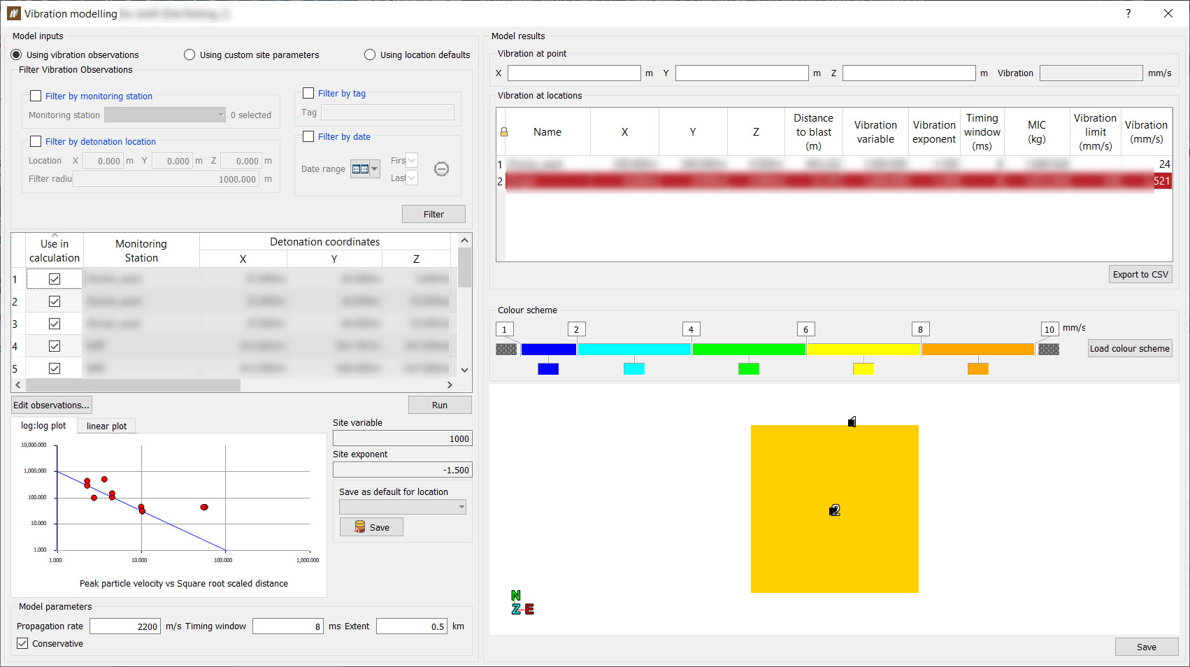
Model inputs and outputs
Vibrations can be calculated either by using vibration observations, custom site parameters or location defaults.
The user is able to filter vibration observations according to the following criteria:
- Filter by monitoring station
- Filter by tag
- Filtered by detonation location
- Filter by date
Custom site parameters
Vibrations can be live edited by modifying the site dependent and exponent which become editable using this option. The values can be saved as the default values for a selected location.
Location defaults
This option automatically changes the Vibration at locations table in Model results to display the Vibration variable and Vibration exponent using the values from their appropriate location. Vibrations will not be calculated at a location which does not have a default variable and exponent. The vibration surface view is removed in this mode.
Conservation check box
When calculating PPV, users can choose to use a weighted distance or the minimum distance (conservative approach). The weighted distance has been included as it more accurately represents the contributing detonations.
 Overpressure Modelling
Overpressure modelling predicts the peak sound pressure caused by a shock wave over and above normal atmospheric pressure measured in decibels (dB). It is calculated in a similar way to vibration with the following differences:
- Independent site variable and site exponent defined in site settings.
- Incorporates wind velocity (only very significant winds will affect the result).
- Has a lower propagation rate (as sound travels faster in rock than in air).
- Formula uses the cube root of charge mass than the square root.
To open the Overpressure Modelling panel, go to Analysis > Vibration > ![]() Overpressure Modelling.
Overpressure Modelling.
Model inputs
Overpressure is dependent on a number of variables, including explosive mass, explosive timing and wind speed and direction. BlastLogic enables the user to enter the following inputs:
-
Propagation rate — The speed of sound through the current atmospheric. This generally taken to be 340m/s, but can vary significantly due to temperature and altitude.
-
Extent — The distance to evaluate from the blast. Larger extents will require longer calculation times.
-
Window direction — The predicted travel direction of the wind at the moment of firing.
Calculation of overpressure
Overpressure at a particular location is calculated using the following procedure:
-
Collect and order each detonation event or time.
-
Calculate the total explosive mass and minimum distance to the point of interest at each detonation event. Adjust the distance values according to wind speed and speed of the sound wave.
-
Calculate the overpressure in kPa for each total explosive mass and minimum distance to the point of interest using the following equation (referenced in the Australian Standards (AS) 2187.2, 2006):
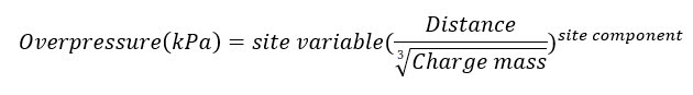 , where the site variable and site exponent are constants set in Setup > Site > Locations.
 -
Convert the value into decibels using the following equation:
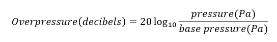 , where the base pressure = 0.00002Pa (or 20µPa)
Background model information
In the basic case scenario, with 1 hole fired and no wind interference, the maximum instantaneous charge (MIC) is calculated from the explosive mass in the hole and value of overpressure for each point on the grid is calculated using the cube root scaled distance formula.
When there are multiple holes, each hole is assigned an initiation time which is equivalent to the initiation time of the first primer in the hole.
For each point in the grid, the propagation rate and initiation time per hole are then used to determine which holes are interacting with each other by taking in consideration the time for overpressure wave to reach the point (ie, distance / propagation rate) and an assumed 8ms window.
The charge mass is thus calculated to be sum of all the charge masses of all the holes whose overpressure waves reaches the same grid point within the 8ms window.
The MIC is calculated as the maximum of these charge mass sums. This is then used in the cube root scaled distance formula to calculate the overpressure value at the given point.
Wind will affect the time taken for the overpressure wave to reach any given. The wind speed is directly added as a velocity component to the wave emanating from a hole.
Important: As the initiation time of a hole is required to work out the interaction of the overpressure waves originating from different holes, any hole that is not a part of a tie-up will be ignored by the modelling tools. Also holes that have no charge plan will have no effect on the model as they have no charge mass.
How to use the Overpressure Modelling tool
Where?
To open the Overpressure Modelling panel, go to the Blast modelling drop-down menu and select Overpressure.
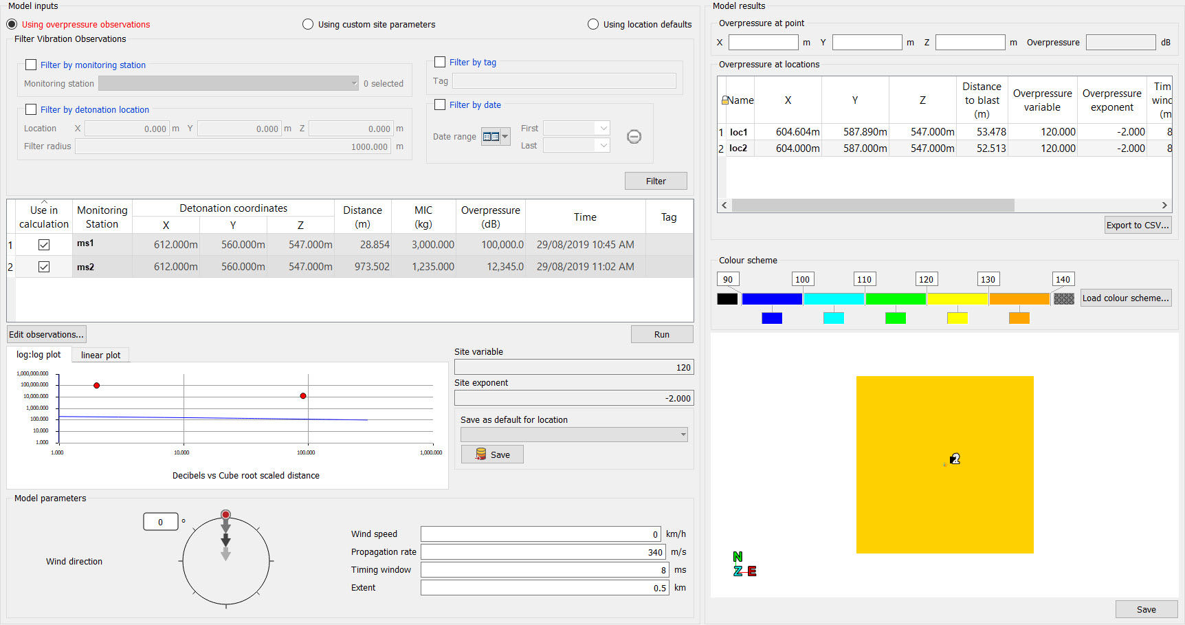
Panel overview
This panel provides a visual tool to model the overpressure effects of a blast.
Custom colour schemes
Custom colour schemes created in the Site > Setup > Custom Colour Schemes panel can be loaded into the Overpressure modelling panel by clicking the Load colour scheme button. The colours and intervals can be further edited in the Overpressure modelling panel. Once a user is happy with what they have created, the scheme can be copied via right click and pasted into the Custom Colour Schemes panel where it can be saved and used again.
Estimating Overpressure
The colour map will allow the user to quickly evaluate the range of overpressures values from the blast within the specified extent.
Note: To save the plot, press the Save button. This will created two new objects in the cad folder: a grid of the plot and a contours map showing intervals in 5dB increments.
Estimating Overpressure at a Point (x,y,z)
To verify overpressure at a specific point the user can enter x,y,z, co-ordinates at the bottom of the panel (for known monitor locations or sensitive areas) or simply click mouse click inside a co-ordinate field and click anywhere on the plot: the x,y,z co-ordinates for the selected point will be displayed. The overpressure at the point will be shown on the right side of the panel.
Estimating Overpressure at locations
The table lists all locations for the site which are within the extent (defined in Setup > Site > Locations) and lists the overpressure calculated from the model at the coordinates of the location. If the overpressure result exceeds the overpressure limit (defined in Setup > Site > Locations), then the row will be highlighted in red.
Clicking Export locations will export the list of locations and their overpressure value to a CSV file.
 Fragmentation Modelling
To open the Fragmentation modelling panel, go to Analysis > Fragmentation > ![]() Fragmentation Modelling.
Fragmentation Modelling.
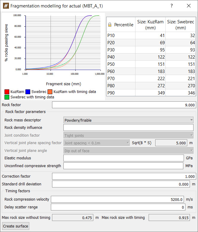
The Fragmentation model panel displays and S-Curve graph with and without timing data obtained from the tie-up. A rock factor is calculated based on the rock factor parameters. Users are also able to explicitly specify a value for a rock factor.
The shape of the S-Curve graph can be modified by altering correction factors. Timing factors also affect the timing data curves.
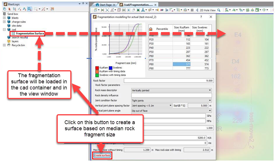
By clicking the Create surface button, you can generate a surface which gives a visual representation of average fragmentation size over the blast. This is based on the charge energy in each hole.
Model inputs
Fragmentation of rock depends on explosive mass and explosive timing, as well as various different rock factors.
The rock factor quantifies the impact of a single rock or rock mass properties on blasting outcomes:
- Rock mass description (RMD) — Select the value that best describes the condition of the rock. The options are:
- Powdery/friable
- Massive formation
- Vertically jointed
- Rock density influence (RDI)— It's estimated as RDI = 25(D) - 50. Where 'D' is the rock mass density in tonnes per cubic metre (t/m3).
- Joint condition factor — Select the options that best describes the conditions of joints in the rock mass. Options are:
- tight joints
- relaxed joints
- gouge-filled joints.
- Vertical joint plane spacing factor (JPS) — This value is partly related to absolute spacing and partly related to the ratio of hole spacing. Select the size of the joint spacing, referencing the calculated hole spacing ratio displayed to the right of this field.
- Vertical joint plane angle or orientation (JPO) — Describes the angle (or orientation) of the joint. The options for this value are:
- Dip out of face
- Strike out of face
- Dip into face.
Dip describes a steep dip of > 30 degrees. 'Out of face' should be used when the extension of the joint plane from the vertical face is upwards.
- Elastic modulus (E)— or Young's modulus is calculated as the ratio between the axial stress and axial strain change in Gigapascals (GPa) . E = Stress / Strain.
- Uniaxial compressive strength (UCS)— is the most widely recognized measure of the strength, deformation and fracture characteristics of the rock in megapascals (MPa). This value is determined by a standard laboratory test which consists of loading a cylindrical sample of the rock with a diameter of 50mm and and length to diameter ratio of 5:2 axially until the specimen fails.
-
Correction factor — After a rock factor is entered or calculated from the parameters, a correction factor can be applied to account for specific site or pit conditions (as the rock factor alone is unable to cater for all possible values). The correction factor should be calibrated and updated once results have been measured.
-
Timing factors — These values are only applicable if the fragmentation model is being run for a tie-up.
-
Rock compression velocity — The compressional stress wave velocity of the rock. This value is used to internally calculate an optimum interhole delay time, based on an optimum interhole delay time of 3-6ms per metre burden.
-
Delay scatter range — Describes the potential range of delay scatter of the initiation system. For electronic tie-up, this value will likely be 0.
Note: Entering the rock factor parameters simply update the “Rock factor” value. It is a more quantifiable way to calculate the rock factor. If the rock factor is already know, it can simply be entered on its own.
Estimating fragmentation
The displayed plot will provide an estimation of the expected proportions of resulting fragmentation of the rock. The maximum expected rock size is shown at the bottom of the panel. If there is timing data provided (ie, the fragmentation model is generated from a tie-up and the timing factors have been set), then there will be a second set of plotted lines, showing how the currently specified tie-up is estimated to affect the fragmentation.
Note: The Swebrec© function simply acts as a replacement for the Rosin-Rammler portion of the Kuz-Ram model. The median and maximum rock sizes are still computed using the adapted Kuznetsov equation found in the Kuz-Ram model.
Note: To see the median rock fragment size as it changes over the blast, press the Create surface button. This will create a surface in the cad container. This surface represents the median rock fragment size without timing data.
 Fly Rock Modelling
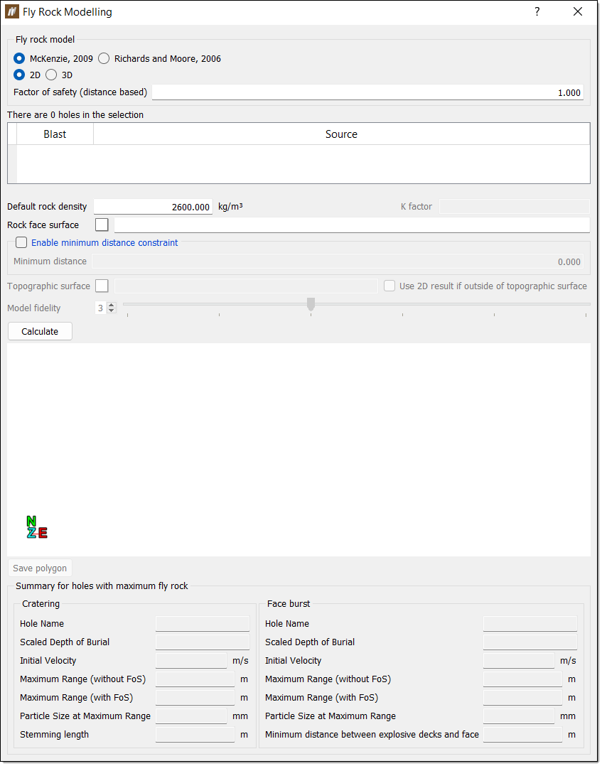
The fly rock model provides a method to predict a maximum horizontal distance of fly rock based on model inputs. The resulting boundary may be used to assist with understanding the potential extent of fly rock displacement and determining blast exclusion zones.
To open the Fly Rock Modelling panel, go to Analysis > Fly Rock > ![]() Fly Rock Modelling. The Fly Rock Modelling panel will appear.
Fly Rock Modelling. The Fly Rock Modelling panel will appear.
Methods
BlastLogic uses kinematic equations from two different methods to calculate fly rock displacement:
-
McKenzie, C.K, 2009. Fly rock range and fragment size prediction, International Society of Explosive Engineers, 35th Annual Conference, Denver, USA.
-
Richards and Moore, 2006. Sourced from the Terrock Supplementary Modelling Report for Kalgoorlie Consolidated Mine.

When using the McKenzie method, we have assumed a particle shape factor of 1.2. This value is the average value for particle shape distribution and is used for determining the effects of air resistance.
Types of fly rock modelling
There are two types of modelling - 3D and 2D models. Both modelling types use a projectile velocity. The velocity is determined from either the McKenzie or Richards and Moore kinematic methods.
In 3D modelling, the velocity is used to calculate the intercept between the trajectory of the rock and the topographic surface provided. This is repeated for a number of vertical angles until the furthest horizontal distance is found for a given orientation. This is then repeated at various orientations in order to form a boundary around each selected hole. After boundaries around individual holes are created, an overall boundary is generated.
In 2D modelling, it is assumed that the topographic surface is flat and therefore that the maximum trajectory angle is 45 degrees. The velocity is used to determine the intercept with this theoretical surface.
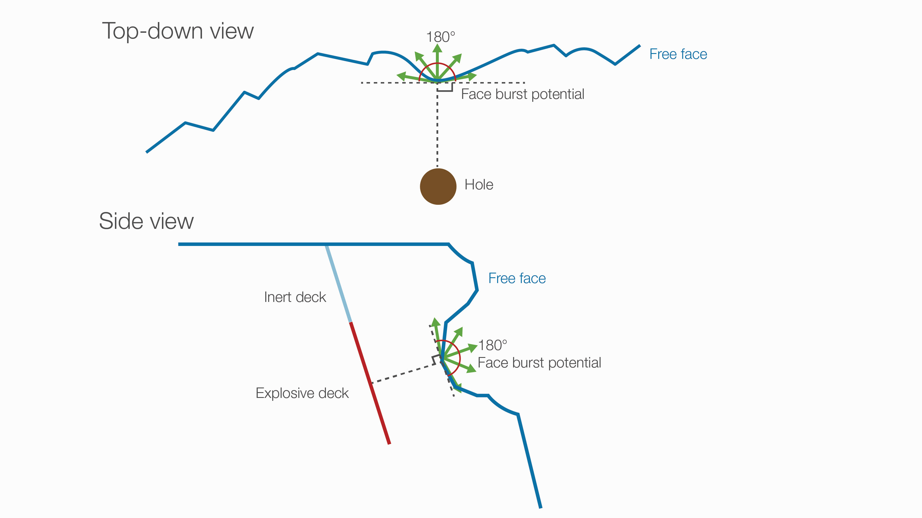
There are two components to fly rock that the model considers: cratering and face burst.
Cratering refers to fly rock from the collar of the hole and directly depends on the amount of stemming in the hole. The more stemming, the lower the amount of cratering.
Only the top-most explosive deck is considered when modelling cratering.
The length of any inert decks (including air) that are above the first explosive deck are considered to contribute to the stemming length.
Face burst refers to fly rock from a free face (generally a highwall) which is provided by the user as a triangulation. The greater the distance between an explosive deck and the triangulation surface, the lower the amount of face burst.
BlastLogic determines a vector of the closest distance between explosive decks and the free face and then models this face burst potential in an arc 180 degrees along the line perpendicular to the vector between the deck and the face. Therefore, if a single hole has two different points that are close to the face, only the closest one will be assessed.
Note that rifling is not currently considered in any model.
Input parameters
There are eight input parameters:
-
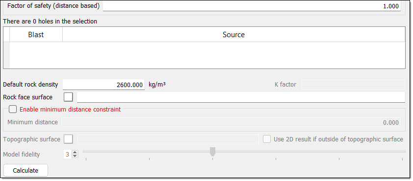
Factor of safety
Both 2D and 3D models use a factor of safety when calculating fly rock. However, when it comes to applying the factor of safety, there are some differences between the two models:-
When calculating the 2D model, the factor of safety is a multiplier applied to the model calculated fly rock horizontal distance.
-
When calculating the 3D model, the factor of safety is a multiplier applied to the initial velocity of the dominant type of fly rock (cratering or face burst).
-
-
Blast and data source
Specify the blast you wish to model in the data explorer or view window. The selection table in the panel will display the selected blast in the Blast column and set the source data to Current in the Source column.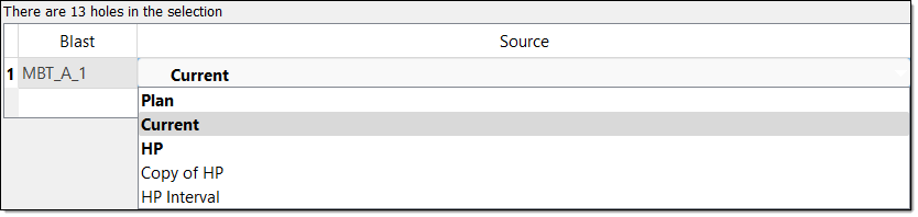
Optionally, change the data source by selecting the Source drop-down and selecting one of the following sources:
-
Plan
Select the Plan option to generate a model using only charge plan data. In this case, no loaded or reconciled data is included in the model. This option is in bold to signify that it is a special data type that you can only access in the tie-up editor and fly rock modelling tool. -
Current
Select the Current option to generate a model using reconciled data. If there is no reconciled data, BlastLogic will load the plan data instead (but not any loaded data). This option is in bold to signify that it is a special data type and not a snapshot -
Reference design snapshot
The name of the reference design snapshot will appear as an option in the drop-down. For example, the snapshot HP, is in bold to represent that it is the reference design snapshot. Select this option to generate a model using the reference design snapshot data. -
Other snapshots
Any other snapshots related to the blast will also appear in the drop-down. Select the name of the desired snapshot to generate a model using that snapshot’s data. These snapshots will not be in bold.
-
-
Density
The McKenzie method uses density to calculate fly rock. If no general average density is provided in the panel, BlastLogic requires the density assigned to each individual hole to calculate fly rock. -
K factor
The Richards and Moore method uses a K factor derived from experimentation. -
Rock surface face
For face burst modelling, a rock face surface is used to calculate the distance between the closest explosive deck and the rock face surface. If no surface is provided, face burst is not considered.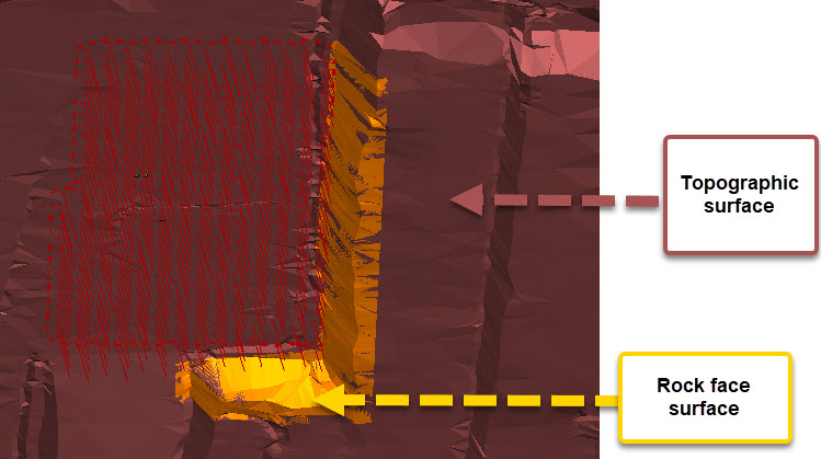
-
Minimum distance constraint
The Enable minimum distance constraint checkbox is used to ensure that the fly rock boundary in any direction will be a user-defined minimum distance. -
Topographic surface
For 3D Modelling, a topographic surface is used to determine the intercepts for both cratering and face burst modelling. The topographic surface should cover the entire extent of both the blast itself and the potential fly rock zone. -
Model fidelity
Model fidelity can be used to modify the number of sampling points used to generate a result. For example, increasing the fidelity will increase the number of orientations and vertical angles considered by the model. The higher the fidelity, the longer the algorithm will take.
Outputs
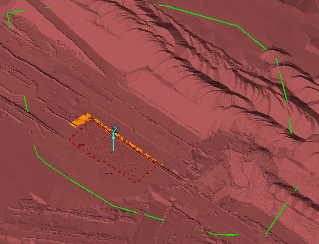
BlastLogic creates an overall flyrock boundary using the maximum horizontal distance from each selected hole.
Cratering and face burst are calculated and displayed separately for the 2D model option. Cratering is displayed as a green boundary, while face burst is displayed as a light blue boundary.
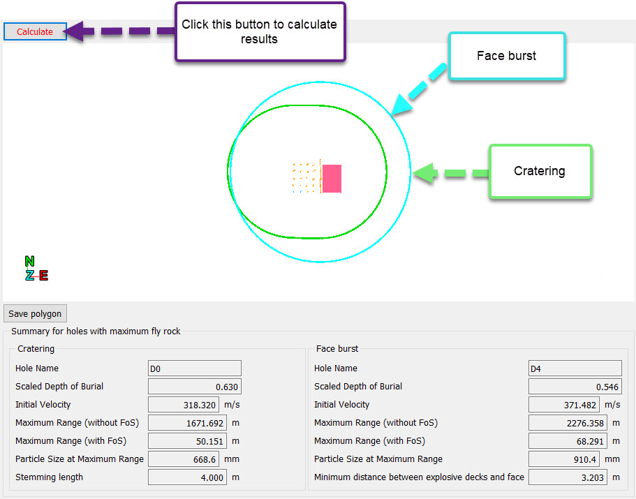
The two results are combined when producing a 3D model. If the boundary doesn’t intersect with the topographic surface, the algorithm will use values calculated from the 2D model.
Fly rock boundaries can be saved by clicking the Save polygon button.