Scans
A scan object represents lidar A method for calculating distances by measuring the time taken for reflected light from laser pulse to return to the receiver. data acquired from a 3D laser scanner. A scan consists of many individual points, each of which corresponds to a single return from the laser scanner. Stationary laser scanners typically acquire data in vertical columns as the scanner head rotates horizontally. For this reason, lidar data is encoded within the scan using spherical coordinates. This means that each point is defined by the following three values:
-
Azimuth. This is also called the horizontal angle.
-
Elevation. This is also called the vertical angle.
-
Range. This is the distance from the scanner’s origin to the measured point.
From the perspective of the scanner, the set of points acquired can be viewed as a grid structure, with each point sitting within a single grid cell. Scans can be connected such that the topological relationship between adjacent points in the grid is acknowledged, or disconnected, so that the grid structure is ignored. Scans can thus be viewed and operated on either as point clouds or as grid structures, depending on the required application.
Important: Examples provided on this page assume experience and knowledge with NumPy arrays, vectorised operations and broadcasting. If you are a beginner please start with examples in Point Sets.
Scan properties
Scan defines the following special properties:
| Property | Description |
|
Use this property to set or return the distance between each point and the origin. This property is represented as an array of float distances. Once the save() function has been called on the Scan object, point_ranges becomes a read-only property. |
|
| Use this property to set or return the azimuth of each point in a scan measured clockwise from the Y axis. Once the save() function has been called on the Scan object, horizontal_angles becomes a read-only property. | |
| Use this property to set or return the elevation angle for each point in a scan. Once the save() function is called on the Scan object, vertical_angles becomes a read-only property. | |
| Use this property to return the total number of rows within a scan. | |
| Use this property to return the total number of columns within a scan. | |
| Use this to set the origin of a scan. It is represented by a single point. If not provided, then the origin will be set to the default value of [0,0,0]. | |
| Use this property to set the maximum range the scanner is capable of. This is used to normalise the ranges to allow for more compact storage. When the save() function is called, any point further away from the origin than max_range will have its range set to max_range. By default, max_range is set to the maximum distance between a point and the origin. | |
| Use this property to set the validity of each cell point within a scan. cell_point_validity is an array of boolean values (True or False) for each cell point. | |
| Use this property to set the intensity of each point in a scan. point_intensity is an array of 16 bit unsigned integers in the range [0, 65535]. | |
| Use this property to return a boolean value indicating if the Scan object is stored within a column-major cell network. | |
| Use this property to query the row and column indices for a given point index. | |
| Use this property to query the index of a point at a grid location specified by a row and column index. |
Scan objects offer similar capabilities to PointSet, however note the following:
- Points within scans can't be translated or removed once the object is created. However you can translate and rotate an entire object (e.g. for registration purposes) and manipulate colours.
- You control point visibility using visibility masks exclusively (as opposed to optionally with PointSet where you can also simply delete points).
- Scans have an intensity property, which is understood by various software features as intensity from a laser return signal.
- Cartesian coordinates are derived from polar coordinates; however you can create and interact with a Scan object using Cartesian coordinates exclusively.
- Many filter examples demonstrated on this page will also be compatible with PointSet, except where scan-only properties are the point of interest, such as point_ranges or point_intensity.
Attributes may be applied to the point primitives also, which can be used for analysis, filtering or colouring purposes while using the SDK.
Some examples in this page use libraries not installed by default. The libraries referenced are:
You may need to install these libraries into your Python environment. To do this, use: python.exe -m pip install library_name
Creating a scan
Basic example
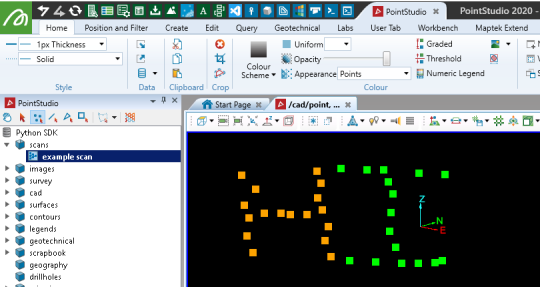
This is a basic example to show how to create a scan using a predefined list of Cartesian coordinates and colours. Once the Scan object has been created, the points can't be deleted or individually transformed. If you need to delete or transform your points, we recommend that you use a PointSet.
from mapteksdk.project import Project
from mapteksdk.data import Scan

proj = Project() # Connect to default application

points = [[-2.1,3.2,4.0],[-1.7,2.9,4.0],[-1.4,2.4,4.0],[-1.1,2.1,4.0],[-0.7,1.6,4.0],
[-0.3,1.2,4.0],[-1.1,2.3,4.0],[-1.0,2.4,4.0],[-0.9,2.4,4.0],[-0.8,2.5,4.0],
[-1.7,3.7,4.0],[-1.4,3.4,4.0],[-1.1,3.0,4.0],[-0.8,2.7,4.0],[-0.4,2.3,4.0],
[-0.1,1.9,4.0],[0.3,1.5,4.0],[-1.6,3.9,4.0],[-1.4,4.0,4.0],[-1.3,4.1,4.0],
[-1.0,4.2,4.0],[-0.8,4.3,4.0],[-1.0,3.8,4.0],[-0.7,3.5,4.0],[-0.3,3.0,4.0],
[0.1,2.5,4.0],[0.5,2.1,4.0],[0.5,1.5,4.0],[0.7,1.6,4.0],[0.9,1.7,4.0],
[1.0,1.8,4.0],[1.1,1.9,4.0],[1.1,2.0,4.0]]

colours = [[255,165,0,255],[255,165,0,255],[255,165,0,255],[255,165,0,255],[255,165,0,255],
[255,165,0,255],[255,165,0,255],[255,165,0,255],[255,165,0,255],[255,165,0,255],
[255,165,0,255],[255,165,0,255],[255,165,0,255],[255,165,0,255],[255,165,0,255],
[255,165,0,255],[255,165,0,255],[0,255,0,255],[0,255,0,255],[0,255,0,255],
[0,255,0,255],[0,255,0,255],[0,255,0,255],[0,255,0,255],[0,255,0,255],
[0,255,0,255],[0,255,0,255],[0,255,0,255],[0,255,0,255],[0,255,0,255],
[0,255,0,255],[0,255,0,255],[0,255,0,255]]

with proj.new("scans/example scan", Scan, overwrite=True) as new_scan:
    new_scan.points = points
    new_scan.point_colours = colours
Creating scans with rows and columns
When a scan is created without any arguments, the points of the scan are considered to be arranged in a grid with one row and point_count columns. This is a degenerate grid that contains no cells. This is not ideal for scans, which have an underlying grid structure. As of mapteksdk 1.3 it is possible to create scans with the points arranged into the specified number of rows and columns. Such scans have the following properties:
-
They have cell properties (see Scan properties)
-
They support invalid points for which point properties are not stored
-
The point count is fixed to (row_count * column_count) - invalid_point_count. Assigning too few or too many points will raise an error.
The example below demonstrates creating a scan with rows and columns.
import numpy as np

from mapteksdk.project import Project
from mapteksdk.data import Scan

# The scan points are arranged into 20 rows and 40 columns.
dimensions = (20, 40)

# Calculate the horizontal angles.
row_start = -np.pi / 4
row_diff = np.pi / 2
row = np.arange(row_start, row_start + row_diff, row_diff / dimensions[1])
horizontal_angles = np.zeros((np.product(dimensions)), dtype=np.double)
horizontal_angles_2d = horizontal_angles[:].reshape(dimensions)
horizontal_angles_2d[:] = row

# Calculate the vertical angles.
col_start = -np.pi / 4
col_diff = np.pi / 2
col = np.arange(col_start, col_start + col_diff, col_diff / dimensions[0])
vertical_angles = np.zeros((np.product(dimensions)), dtype=np.double)
vertical_angles_2d = vertical_angles[:].reshape(dimensions)
vertical_angles_2d.T[:] = col

project = Project()

with project.new(
    "scans/row_col_scan",
    Scan(dimensions=dimensions), overwrite=True) as scan:
  scan.horizontal_angles = horizontal_angles
  scan.vertical_angles = vertical_angles
  scan.point_ranges = 100
|
|
|
The resulting scan. |
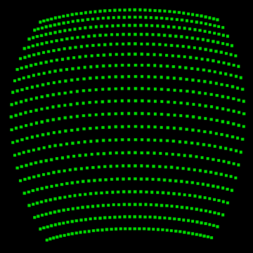
Note the following about the scan in this example:
-
The points of the scan are arranged in 20 rows and 40 columns, the same as the dimensions parameter passed to the constructor. This grid structure of the points is required when creating scans with rows and columns.
-
The angles of the points are evenly spaced. This matches how many lidar scanners generate scans.
-
All of the range values in the scan are the same, meaning all points are located on a sphere centred on the location of the scanner. More complicated scans are constructed by varying the range values.
Scans with more rows and columns can represent more detail.
Cell point validity
In the previous example every point in the grid has a point. This is unrealistic for real scan data. For example, when scanning the topography of an area often there is nothing to scan at the higher points. Because there was nothing to scan, there should be no point at that location in the grid. To handle this, scans have the concept of “point validity”, which allows for the grid of points to contain holes/gaps.
In a scan where all points are valid, the point count is equal to row_count * column_count. In a scan with invalid points, the point count will be less than row_count * column_count.
The cell_point_validity array is an array containing row_count * column_count values. True indicates the point is valid and False indicates the point is invalid.
The following table lists the commonalities and differences between valid and invalid points:
| Valid points | Invalid points | |
|---|---|---|
| Have cell point properties, such as Scan.horizontal_angles and vertical_angles | ✓ | ✓ |
| Have point attributes, such as point_colours and point_ranges | ✓ | ✗ |
The following example demonstrates creating a scan with invalid points.
from mapteksdk.project import Project
from mapteksdk.data import Scan

dimensions = (5, 5)

horizontal_angles = [
  -0.28, -0.14, 0., 0.14, 0.28,
  -0.28, -0.14, 0., 0.14, 0.28,
  -0.28, -0.14, 0., 0.14, 0.28,
  -0.28, -0.14, 0., 0.14, 0.28,
  -0.28, -0.14, 0., 0.14, 0.28,]

vertical_angles = [
  -0.28, -0.28, -0.28, -0.28, -0.28,
  -0.14, -0.14, -0.14, -0.14, -0.14,
  0., 0., 0., 0., 0.,
  0.14, 0.14, 0.14, 0.14, 0.14,
  0.28, 0.28, 0.28, 0.28, 0.28,]

point_validity = [
  False, False, True, True, False,
  False, True, True, False, False,
  True, True, True, True, False,
  True, True, True, True, True,
  False, True, True, True, False,]

# Point properties only have values for valid points.
point_ranges = [
  22, 24,
  18, 21,
  16.8, 19, 22, 26,
  17.5, 21, 23, 25, 31,
  20, 20.5, 23,]

point_intensity = [
  36699, 34078,
  41942, 38010,
  44563, 40631, 36699, 31456,
  43253, 38010, 35388, 32767, 24903,
  39321, 39321, 35388,]

project = Project()

with project.new("scans/small_invalid_points_scan",
    Scan(dimensions=dimensions,
         point_validity=point_validity)) as scan:
  scan.vertical_angles = vertical_angles
  scan.horizontal_angles = horizontal_angles
  scan.point_ranges = point_ranges
  scan.point_intensity = point_intensity
  scan.max_range = 100
|
|
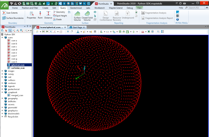
Creating with spherical coordinates
This example creates a Scan using spherical coordinates to define the point locations (using the point_ranges, horizontal_angles and vertical_angles arrays). When dealing with raw laser scan data it may be provided in this form and can be used as an alternative to Cartesian coordinates (with less loss of precision).
import numpy as np
from mapteksdk.project import Project
from mapteksdk.data import Scan
from numpy import pi, cos, sin, arccos, arange, arctan2, sqrt

project = Project()
radius = 15
num_pts = 3000
origin = [50, 0, 0]

with project.new("scans/spherical_scan", Scan, overwrite=True) as new_scan:
    indices = arange(0, num_pts, dtype=np.float64) + 0.5
    phi = arccos(1 - 2*indices/num_pts)
    theta = pi * (1 + 5**0.5) * indices
    x, y, z = (cos(theta) * sin(phi))*radius, (sin(theta) * sin(phi))*radius, cos(phi)*radius

    new_scan.point_ranges = sqrt(x**2 + y**2 + z**2)
    new_scan.horizontal_angles = np.arctan2(y, x)
    new_scan.vertical_angles = np.arctan2(z, sqrt(x**2 + y**2))
    new_scan.save() # Save to initialise the default colour array
    new_scan.point_colours[:] = [255, 0, 0, 255] # Set the colour
    new_scan.origin = origin
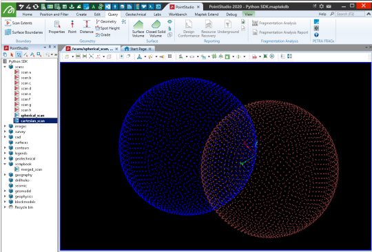
Creating with Cartesian coordinates
This example creates a scan using the same points as the spherical example, but provided in Cartesian form. The location is slightly offset so the two scans can easily be viewed for differences. There is a slight loss in precision when creating a scan from Cartesian coordinates and they are converted in the background to spherical coordinates.
Creating a Scan object from Cartesian coordinates is offered for convenience and operates similarly to the ASCII importer in PointStudio and Vulcan GeologyCore. When using Cartesian coordinates, they are written as a single row of points with the number of columns matching the number of points (this affects tools like Scan Connectivity as the scan is not properly represented as a form of a irregular grid).
import numpy as np
from mapteksdk.project import Project
from mapteksdk.data import Scan
from numpy import pi, cos, sin, arccos, arange

project = Project()
radius = 15
num_pts = 3000
origin = [60, 15, 10]

with project.new("scans/cartesian_scan", Scan, overwrite=True) as new_scan:
    indices = arange(0, num_pts, dtype=float) + 0.5
    phi = arccos(1 - 2*indices/num_pts)
    theta = pi * (1 + 5**0.5) * indices
    x, y, z = (cos(theta) * sin(phi))*radius, (sin(theta) * sin(phi))*radius, cos(phi)*radius

    new_scan.points = np.column_stack((x,y,z))
    new_scan.save() # Save to initialise the default colour array
    new_scan.point_colours[:] = [0, 0, 255, 255] # Set the colour
    new_scan.origin = origin
Creating from a ply point cloud
This example demonstrates creation of a scan from an input .ply file containing a point cloud.
Important: This makes use of the open3d library, which is not included by default with Python. You may need to install it before trying the script.
import os
import numpy as np
from mapteksdk.project import Project
from mapteksdk.data import Scan
from typing import Tuple

def open3d_ply_importer(file_path:str) -> Tuple[np.ndarray, np.ndarray]:
    """Loads a ply file into memory with open3d and returns (points, colours).
    Args:
        file_path (str): path to .ply point cloud file
    Returns:
        Tuple[np.ndarray, np.ndarray]: (points, point_colours)
    """
    import open3d as o3d
    pcd = o3d.io.read_point_cloud(file_path, format="ply", print_progress=True)
    points = np.asarray(pcd.points, dtype=np.float64)
    # make a default colour array
    rgba = np.full((points.shape[0], 4), 255, dtype=np.uint8)
    # check if the point cloud has colours
    pcd_colors = np.asarray(pcd.colors)
    if pcd_colors.shape[0] == points.shape[0]:
        # open3d colours are 0-1 floats, need to convert to 0-255 uint8
        rgba[:, 0:3] = (pcd_colors * 255).astype(np.uint8)
    return (points, rgba)

def pyntcloud_ply_importer(file_path:str) -> Tuple[np.ndarray, np.ndarray, np.ndarray]:
    """Loads a ply file into memory with pyntcloud and returns (points, colours, intensity).
    Args:
        file_path (str): path to .ply point cloud file
    Returns:
        Tuple[np.ndarray, np.ndarray, np.ndarray]: (points, point_colours, point_intensity)
    """
    from pyntcloud import PyntCloud
    ply = PyntCloud.from_file(file_path)
    # convert all columns to lower case as things like scalar_intensity could be scalar_Intensity
    ply.points.columns = ply.points.columns.str.lower()
    intensity = np.zeros((ply.xyz.shape[0],1), dtype=np.uint32)
    rgba = np.full((ply.xyz.shape[0],4), 255, dtype=np.uint32)
    if "scalar_intensity" in ply.points:
        intensity = ply.points["scalar_intensity"].to_numpy(dtype=np.uint32)
    if "red" in ply.points:
        rgba[:,0] = ply.points["red"].to_numpy(dtype=np.uint8)
    if "green" in ply.points:
        rgba[:,1] = ply.points["green"].to_numpy(dtype=np.uint8)
    if "blue" in ply.points:
        rgba[:,2] = ply.points["blue"].to_numpy(dtype=np.uint8)
    return (ply.xyz, rgba, intensity)

if __name__ == "__main__":
    file_path = ""
    while not os.path.isfile(file_path):
        file_path = input("Enter ply file path:\n")
    save_path = os.path.basename(file_path)

    proj = Project() # Connect to default project
    try:
        with proj.new(f"scans/{save_path}", Scan, overwrite=True) as scan:
            scan.points, scan.point_colours, scan.point_intensity = pyntcloud_ply_importer(file_path)
        print(f"Saved scans/{save_path}")
    except Exception as ex:
        print(f"An error occurred: {ex}")
Creating from a PLY point cloud using a workflow
The following example creates a scan from a PLY file (.ply) containing a point cloud. It uses Python for the import process as well as a range of functionality to illustrate how the SDK can be used in conjunction with a Maptek workflow to provide a user-facing tool for executing it.
Important: This makes use of the pyntcloud library, which is not included by default with Python. You may need to install it before trying the script. However, when the user runs the workflow, if they don’t have the required dependency on the pyntcloud library, it will attempt to be installed automatically using pip.
Reading of the PLY file is performed using pyntcloud instead of open3d as per the last example, as pyntcloud will also support intensity data if the point cloud has it.
import os
import subprocess
import sys
import numpy as np
from mapteksdk.project import Project
from mapteksdk.data import Scan, Container
from typing import Tuple
from mapteksdk.workflows import WorkflowArgumentParser

def pyntcloud_ply_importer(file_path:str) -> Tuple[np.ndarray, np.ndarray, np.ndarray]:
    """Loads a ply file into memory with pyntcloud and returns (points, colours, intensity).
    Args:
        file_path (str): path to .ply point cloud file
    Returns:
        Tuple[np.ndarray, np.ndarray, np.ndarray]: (points, point_colours, point_intensity)
    """
    try:
        from pyntcloud import PyntCloud
    except ImportError:
        try:
            subprocess.call([sys.executable, "-m", "pip", "install", "pyntcloud", "--user"])
            from pyntcloud import PyntCloud
        except ImportError:
            input("There was an error importing/installing 'pyntcloud'.\n"
            + "Please run 'python -m pip install pyntcloud' to install a necessary package.")
            sys.exit(2)
    ply = PyntCloud.from_file(file_path)
    # convert all columns to lower case as things like scalar_intensity could be scalar_Intensity
    ply.points.columns = ply.points.columns.str.lower()
    intensity = np.zeros((ply.xyz.shape[0],1), dtype=np.uint32)
    rgba = np.full((ply.xyz.shape[0],4), 255, dtype=np.uint32)
    if "scalar_intensity" in ply.points:
        intensity = ply.points["scalar_intensity"].to_numpy(dtype=np.uint32)
    if "red" in ply.points:
        rgba[:,0] = ply.points["red"].to_numpy(dtype=np.uint8)
    if "green" in ply.points:
        rgba[:,1] = ply.points["green"].to_numpy(dtype=np.uint8)
    if "blue" in ply.points:
        rgba[:,2] = ply.points["blue"].to_numpy(dtype=np.uint8)
    return (ply.xyz, rgba, intensity)

if __name__ == "__main__":
    parser = WorkflowArgumentParser("Import ply as a scan.")
    parser.declare_input_connector("file_path", str, "", "Path to ply file")
    parser.declare_input_connector("destination", str, "/scans/", "Path to save scan")
    parser.declare_output_connector("selection", list, "Imported scan")
    parser.parse_arguments()

    if not os.path.isfile(parser["file_path"]):
        raise FileNotFoundError(f"File not found {parser['file_path']}")

    proj = Project() # Connect to default project

    # Set the save path for the object. If a container was provided, store inside of it.
    save_path = parser["destination"]
    test = proj.find_object(save_path)
    if save_path.endswith("/") or (test.exists and test.is_a(Container)):
        save_path = f"{save_path}/{os.path.basename(parser['file_path'])}".replace("//","/")

    # Read the ply file and convert to scan object
    with proj.new(save_path, Scan, overwrite=True) as scan:
        scan.points, scan.point_colours, scan.point_intensity = pyntcloud_ply_importer(parser['file_path'])

    # Write list output of path to saved object for Workflow
    parser.set_output("selection", [scan.id.path])
When used in a Workflow, this animation shows how the script is operated:
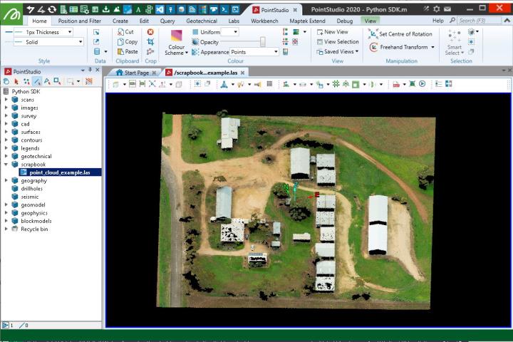
Creating from a Lidar LAS file
This example shows how to create a Scan object by reading a LAS file (.las).
Important: This makes use of the laspy library, which is not included by default with Python. You may need to install it before trying the script.
Note: Data used for this example can be found in Maptek_PythonSDK_Sample_IO_Files_20200108.zip.
import os
import numpy as np
import laspy
from mapteksdk.project import Project
from mapteksdk.data import Scan

proj = Project() # Connect to default project
las_file = r"F:\Python SDK Help\data\point_cloud_example.las"

# Import las format:
with laspy.file.File(las_file, mode="r") as lasfile:
    # Setup valid arrays for storing in a PointSet
    las_points = np.column_stack((lasfile.x, lasfile.y, lasfile.z))

    # Read colour data and prepare it for storing:
    # If the colours have been stored in 16 bit, we'll need to get the first 8 bits for a proper value
    colours_are_16bit = np.max(lasfile.red) > 255
    red = np.right_shift(lasfile.red, 8).astype(np.uint8) if colours_are_16bit else lasfile.red
    green = np.right_shift(lasfile.green, 8).astype(np.uint8) if colours_are_16bit else lasfile.green
    blue = np.right_shift(lasfile.blue, 8).astype(np.uint8) if colours_are_16bit else lasfile.blue
    # Create rgba array
    las_colours = np.column_stack((red, green, blue))

    # Create Scan object and populate data
    import_as = "scrapbook/{}".format(os.path.basename(las_file))

    with proj.new(import_as, Scan, overwrite=True) as scan:
        scan.points, scan.point_colours = (las_points, las_colours)
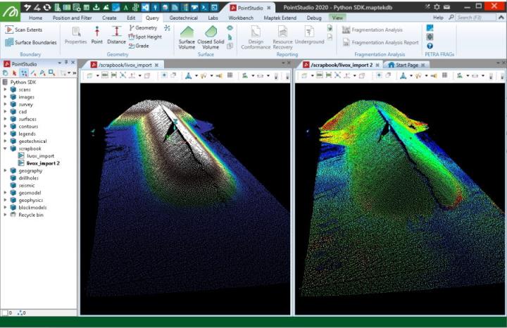
Creating from Livox CSV files
This example takes four CSV files, originating from Livox scanners in format X(mm),Y(mm),Z(mm),intensity that have already know registration values for each the origin position and 3D orientation of each scan. These registration values are applied to the point clouds, along with some basic filtering and colouring then used to create a Scan object. Details on how the registration values were derived for this example (by using PointStudio registration and registration export) are included in the snippet contents. The path for variable scan_pathneeds to be set to where you've extracted the data.
Scipy is used to apply the rotation transforms and matplotlib for generating a colour map used for colouring the points by height.
Note: Data used for this example can be found here: Scan_Create_from_Livox_csv.zip
Important: This makes use of the scipy and matplotlib libraries, which are not included by default with Python. You may need to install them before trying the script.
from mapteksdk.project import Project
from mapteksdk.data import Scan
import numpy as np
import pandas as pd
import matplotlib
import matplotlib.cm as cm
from scipy.spatial.transform import Rotation as R

##### RIGID SCAN REGISTRATION DETAILS ####
# Scan position + rotations - these transforms will put the raw data in the registered positions as
# determined earlier by importing with mm units and globally registering them to where they need to be.
# Scan origins set to 0,0,0 (Labs > Set scan origin) prior to registration (so rotations/translations are relative to 0,0,0 origin).
# Export scan registration (Labs > Registration I/O).
# Use Quaternion from .rqf - PointStudio outputs in w,x,y,z form so need to re-order to x,y,z,w for R.from_quat
# e.g. if the .rqf file has = -0.95,0.034,-0.058,-0.278,-38.77,77.05,1.170
# then from_quat is [0.034,-0.058,-0.278, -0.95] and translation is [-38.77,77.05,1.170]
settings = {}
scan_path = "F:/Python SDK Help/data/livox_scan{}.csv"
settings["scan1"] = (
    scan_path.format("1"),
    R.from_quat([-0.0051625680820143521,0.0057275522235019829,-0.84650225225775189, -0.53232929654385863]), # Rotation
    [14.881705146750189,66.717966400357071,0.070117464411544206] # Translation
    )
settings["scan2"] = (
    scan_path.format("2"),
    R.from_quat([0.0020431597672171068,-0.0032686179056091,0.97364830138733216, 0.22802220690256397]), # Rotation
    [31.013939093526869,140.80530168301951,0.037274415151044571] # Translation
    )
settings["scan3"] = (
    scan_path.format("3"),
    R.from_quat([0.0097925671622976513,-0.0081175702002627623,0.013547158751973432, 0.99982732767821703]),  # Rotation
    [-23.922778199636721,147.18753961890008,1.2875114634996614] # Translation
    )
settings["scan4"] = (
    scan_path.format("4"),
    R.from_quat([0.034888104752663143,-0.058696768275379459,-0.27820153073451415, -0.95809259356169063]),  # Rotation
    [-38.777002133456364,77.053622695856461,1.1703300873891145] # Translation
    )
#####################################

def read_register_csv(scan, unit=0.001):
    # Scan is a tuple(path, rotation, translation)
    file_path = scan[0]
    rotation = scan[1]
    translation = scan[2]
    # Use pandas to read the csv fast, 0=x, 1=y, 2=z, 3=intensity
    csv = pd.read_csv(file_path, delimiter=",", header=None)
    points = csv[[0,1,2]].to_numpy(dtype='float64')
    intensity = csv[3].to_numpy(dtype='uint32')
    # mm -> m
    points = points * unit
    # Apply rotation and translation to csv data to known registered locations and orientations
    points = rotation.apply(points) + translation
    return points, intensity

def topography_filter(points, intensities=None, colours=None, cell_size=0.1):
    # For filtering performance, sort the point data by height
    sorted_indices = points[:, 2].argsort() # sort by z
    points = points[sorted_indices]
    #intensities = intensities[sorted_indices] if intensities is not None else None
    # Create a grid around the data by snapping X and Y values into grid
    filter_pts = pd.DataFrame(points, columns=['X', 'Y', 'Z'])
    filter_pts["X_Grid"] = np.round(filter_pts['X']/cell_size)*cell_size
    filter_pts["Y_Grid"] = np.round(filter_pts['Y']/cell_size)*cell_size
    # head(1) = keep 1st in group (i.e. lowest)
    filtered_indices = filter_pts.groupby(['X_Grid', 'Y_Grid'])['Z'].head(1).index
    # Reset point array to be the filtered points
    # Can also return X_Grid, Y_Grid if you wanted to snap them all to a regular grid
    keep_indices = np.isin(filter_pts.index, filtered_indices)
    points = points[keep_indices]
    intensities = intensities[sorted_indices][keep_indices] if intensities is not None else None
    colours = colours[sorted_indices][keep_indices] if colours is not None else None
    return points, intensities, colours

def colour_by_height(points):
    # Find 5%-95% of z range
    z_range = np.percentile(points[:,2], (5,95))
    # Create a normalise colour map across the range
    norm = matplotlib.colors.Normalize(vmin=z_range[0], vmax=z_range[1], clip=True)
    # https://matplotlib.org/examples/color/colormaps_reference.html
    # Convert to 0-255 RGBA by multiplying the range by 255
    colours = cm.terrain(norm(points[:,2]))*255
    # Convert to uint8
    rgb = colours.astype('uint8')
    return rgb

if __name__ == "__main__":
    proj = Project()
    csv_points = np.empty([0,3], dtype=np.float64)
    csv_intensity = np.empty([0], dtype=np.uint32)

    # Each read_register_csv will return a registered copy of the points
    # np.vstack will concatenate the raw point clouds into one
    for scan in settings:
        points, intensity = read_register_csv(settings[scan])
        csv_points = np.vstack((csv_points, points))
        csv_intensity = np.hstack((csv_intensity, intensity))
    colours = colour_by_height(csv_points)
    # Apply a 0.2m topography filter
    csv_points, csv_intensity, colours = topography_filter(csv_points, csv_intensity, colours, 0.2)

    # Save a copy of the filtered points in PointStudio as a scan
    with proj.new(f"scrapbook/livox_import", Scan, overwrite=True) as points:
        points.points = csv_points
        points.point_intensity = csv_intensity
        points.point_colours = colours
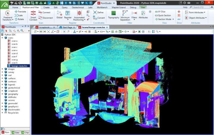
Creating from a Livox LVX file
This example creates a scan from a native Livox LVX format file (.lvx). It uses openpylivox to read the data. Data imported from an LVX file using this snippet may not display in a usable form if it is from a scan where the scanner was moving between frames.
Important: This makes use of the openpylivox and matplotlib libraries, which are not included by default with Python. You may need to install it before trying the script.
from mapteksdk.project import Project
from mapteksdk.data import Scan
import numpy as np
import os
import matplotlib
import matplotlib.cm as cm

# Note: You will need to manually install this library for reading lvx files:
# pip install git+https://github.com/ryan-brazeal-ufl/openpylivox.git
from openpylivox.BinaryFileReader import BinaryReaders
# Lvx sample data available at https://www.livoxtech.com/downloads,
# however this importer may struggle with moving data.

if __name__ == "__main__":
    path = ""
    while not os.path.isfile(path) and not path.lower().endswith(".lvx"):
        path = input("Provide path to Livox lvx file:\n")

    lvx_reader = BinaryReaders.lvxreader(showmessages=False, pathtofile=path)
    lvx_array = np.asarray(lvx_reader.datapoints)
    xyz = lvx_array[:, 0:3].astype(np.float64)
    intensity = lvx_array[:,3].astype(np.uint32)

    proj = Project()
    # Save the points in PointStudio as a scan
    with proj.new(f"scans/{os.path.basename(path)}", Scan, overwrite=True) as scan:
        scan.points = xyz
        scan.point_intensity = intensity
        # Colour by intensity
        i_range = np.percentile(intensity, (1,99))
        # Create a normalise colour map across the range
        norm = matplotlib.colors.Normalize(vmin=i_range[0], vmax=i_range[1], clip=True)
        # https://matplotlib.org/examples/color/colormaps_reference.html
        # Convert to 0-255 RGBA by multiplying the range by 255
        colours = cm.rainbow(norm(intensity))*255
        # Convert to uint8 and store in scan
        scan.point_colours = colours.astype('uint8')
Accessing a scan’s points
Accessing points by row and column index
Unlike GridSurface, Scan objects can contain invalid points, which results in ‘holes’ in the underlying grid structure. This makes it difficult to determine the index of a point given its row and column and vice versa. The Maptek Python SDK offers the Scan.point_to_grid_index and Scan.grid_to_point_index properties, which handle this in an efficient manner.
Point to grid index
A scan’s point to grid index maps the index of a point to its row and column in the scan grid. By way of example, the line of code below assigns the row and column indices of the ith point of the scan to row and column, respectively:
row, column = scan.point_to_grid_index[i]
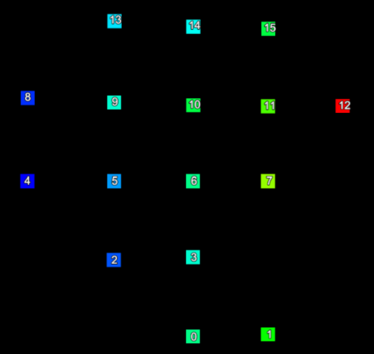
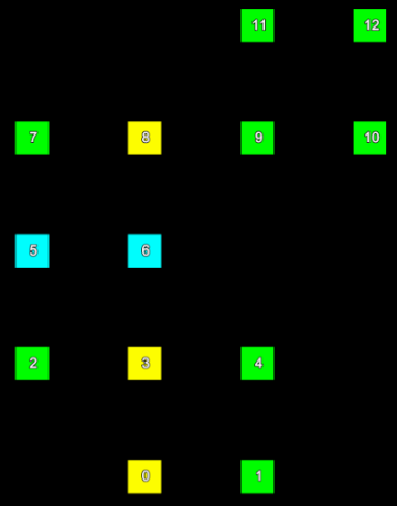
Consider a small section of a scan represented in the two images below. The left hand image shows the index of each point and the right hand image shows the row and column the point is located in the form (row, column).
|
|
|
|
The point indices (left) of a set of scan points and their corresponding grid point indices (right). |
|

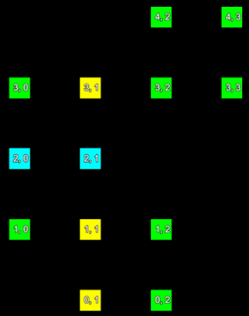
We can represent the information from these images mapping point index to grid (row and column) index in the following table:
| Point index | Row | Column |
|---|---|---|
| 0 | 0 | 1 |
| 1 | 0 | 2 |
| 2 | 1 | 0 |
| 3 | 1 | 1 |
| 4 | 1 | 2 |
| 5 | 2 | 0 |
| 6 | 2 | 1 |
| 7 | 3 | 0 |
| 8 | 3 | 1 |
| 9 | 3 | 2 |
| 10 | 3 | 3 |
| 11 | 4 | 2 |
| 12 | 4 | 3 |
This table essentially expresses the content of the Scan.point_to_grid_index. The following script demonstrates using the point to grid index to generate a boolean array that can be used to index the point properties of a scan to only make changes to points in a specific row or column:
from mapteksdk.project import Project
from mapteksdk.data import Scan, Text2D, HorizontalAlignment, VerticalAlignment

if __name__ == "__main__":
  point_validity = [
    False, True, True, False,
    True, True, True, False,
    True, True, False, False,
    True, True, True, True,
    False, False, True, True
  ]

  with Project() as project:
    path = "scans/point_to_grid_index"
    with project.new(path, Scan(
        dimensions=(5, 4), point_validity=point_validity
        ), overwrite=True) as scan:
      scan.points = [
        [1, 0, 0], [2, 0, 0], [0, 1, 0], [1, 1, 0], [2, 1, 0], [0, 2, 0],
        [1, 2, 0], [0, 3, 0], [1, 3, 0], [2, 3, 0], [3, 3, 0], [2, 4, 0],
        [3, 4, 0]
      ]

      # scan.point_to_grid_index[:, 0] gives the first column of the
      # point_to_grid_index - it is an array of row index for each point.
      # scan.point_to_grid_index[:, 0] == 2 is thus True for every point where
      # the row index is 2.
      row_two = scan.point_to_grid_index[:, 0] == 2
      # This will set all points in row index 2 to Cyan.
      scan.point_colours[row_two] = [0, 255, 255, 255]

      # scan.point_to_grid_index[:, 1] gives the second column of the
      # point_to_grid_index - it is an array of column index for each point.
      # second_column = scan.point_to_grid_index[:, 1] == 1 is thus true for
      # every point where the column index is 1.
      column_one = scan.point_to_grid_index[:, 1] == 1
      # This will set all points in row column 1 to yellow.
      scan.point_colours[column_one] = [255, 255, 0, 255]
Note that:
-
The following code will set index so that if it is used to index into a point property of the scan it will get all points in the ith column:
index = scan.point_to_grid_index[:, 0] == i
-
The following snippet will set index so that if it is used to index into a point property of the scan it will get all points in the kth row:
index = scan.point_to_grid_index[:, 1] == k
-
The results of the above lines can be used with any point property of the scan. This includes the point ranges, point colours, point selection, and point visibility.
-
The results of the above lines cannot be used with cell point properties such as the horizontal/vertical angles, or point validity.
Grid to point index
The grid to point index is the inverse of the point to grid index. It allows for determining the index of a point given that point’s row and column. By way of example, the following line of code sets i to the index of the point in the specified row and column:
i = scan.grid_to_point_index[row, column]
So what if there is no point in the specified row and column? In that case it will be set to the value numpy.ma.masked. This value is a placeholder for an invalid value. Attempting to index into point property arrays with it will raise an error.
For example, using the same scan as in the previous section:
The following table shows the grid to point index with the invalid values marked in red:
| Row | 4 | Invalid | Invalid | 11 | 12 |
| 3 | 7 | 8 | 9 | 10 | |
| 2 | 5 | 6 | Invalid | Invalid | |
| 1 | 2 | 3 | 4 | Invalid | |
| 0 | Invalid | 0 | 1 | Invalid | |
| 0 | 1 | 2 | 3 | ||
| Column | |||||
Note that the grid to point index is a two dimensional array. To read the point index for a specified row and column requires specifying both the row and the column.
Using the grid to point index can be more difficult than using the point to grid index because invalid values must be filtered out before attempting to use it. The following example demonstrates creating the same scan shown above using the grid to point index instead of the point to grid index:
from mapteksdk.project import Project
from mapteksdk.data import Scan, Text2D
import numpy as np

if __name__ == "__main__":
  point_validity = [
        False, True, True, False,
        True, True, True, False,
        True, True, False, False,
        True, True, True, True,
        False, False, True, True
      ]

  with Project() as project:
    path = "scans/grid_to_point_index"
    with project.new(path, Scan(
        dimensions=(5, 4), point_validity=point_validity
        ), overwrite=True) as scan:
      scan.points = [
        [1, 0, 0], [2, 0, 0], [0, 1, 0], [1, 1, 0], [2, 1, 0], [0, 2, 0], [1, 2, 0],
        [0, 3, 0], [1, 3, 0], [2, 3, 0], [3, 3, 0], [2, 4, 0], [3, 4, 0]
      ]

      # scan.grid_to_point_index[:, 1] is an array of the indices of points
      # in the column with index 1.
      column_one = scan.grid_to_point_index[:, 1]
      # Once again filter out the invalid points.
      column_one = column_one[column_one != np.ma.masked]
      # Set all points in the column with index one to yellow.
      scan.point_colours[column_one] = [255, 255, 0, 255]

      # scan.grid_to_point_index[2] is an array of the indices of points
      # in the row with index 2.
      row_two = scan.grid_to_point_index[2]
      # Filter out any element in row_two that is less than zero, because
      # it indicates an invalid point.
      row_two = row_two[row_two != np.ma.masked]
      # Set all points in the row with index two to cyan.
      scan.point_colours[row_two] = [0, 255, 255, 255]

      for row in range(scan.row_count):
        for col in range(scan.column_count):
          if scan.grid_to_point_index.mask[row, col] == True:
            print(f"Skipping: {row} {col} because it is invalid.")
            continue
          point_index = scan.grid_to_point_index[row, col]
          with project.new(path + f"_index_labels/{row}{col}",
              Text2D, overwrite=True) as label:
            label.location = scan.points[point_index]
            label.location[2] += 1
            label.text = str(point_index)
Note that:
-
The following code will set index to the index of the point in the ith row and kth column:
index = scan.grid_to_point_index[i, k]
-
The following code will set index to an array containing the indices of each point in the ith row of the scan (including invalid points):
index = scan.grid_to_point_index[i]
-
The following code will set index to an array containing the indices of each point in the kth column (including invalid points):
index = scan.grid_to_point_index[:, k]
-
The following code filters the invalid point indices from the grid to point index:
index = index[index != np.ma.masked]
-
The results of the above lines can be used with any point property of the scan. This includes the point ranges, point colours, point selection, and point visibility.
-
The results of the above lines cannot be used with cell point properties, such as the horizontal/vertical angles or point validity.
Scan manipulation examples
Translating a scan
To translate a Scan, you need to translate the entire object. This is done by adjusting the origin property.
It is not possible to translate individual points (or the points array, as done with a PointSet) within a scan once it has been created.
from mapteksdk.project import Project
from mapteksdk.data import Scan

proj = Project() # Connect to default project
selection = proj.get_selected()[0] # Get first object in selection
translate_by = [0, 0, 50] # translate in z by +50
if selection.is_a(Scan):
    with proj.edit(selection) as scan:
        # You can't modify 'scan' points directly, but can translate
        # and rotate the origins of the scan.  Here we are translating
        # the origin to cause the entire scan to move.
        scan.origin += translate_by
else:
    print("Select one scan and try again.")
![]()
Colouring by intensity
This example shows how to use the intensity property/data within a scan to colour the points by intensity. A basic colour map from matplotlib.cm is used for colouring, applied across 98% of the data extent and converted to be compatible as a point_colours array.
Important: This makes use of the matplotlib library, which is not included by default with Python. You may need to install it before trying the script.
import numpy as np
from mapteksdk.project import Project
from mapteksdk.data import Scan
import matplotlib
import matplotlib.cm as cm

proj = Project() # Connect to default project

for item in proj.get_selected():
    # Limit filtering to Scan objects as only they contain the point_intensity attribute
    if item.is_a(Scan):
        with proj.edit(item) as scan:
            # Find 1%-99% of intensity range
            # Note: These values can be adjusted to fit into a smaller range
            i_range = np.percentile(scan.point_intensity, (1,99))

            # Create a normalise colour map across the range
            norm = matplotlib.colors.Normalize(vmin=i_range[0], vmax=i_range[1], clip=True)

            # https://matplotlib.org/examples/color/colormaps_reference.html
            # Convert to 0-255 RGBA by multiplying the range by 255
            colours = cm.rainbow(norm(scan.point_intensity))*255
            # Convert to uint8 and store in scan
            scan.point_colours = colours.astype('uint8')
Indicating the volume of a surface on selection
This example pulls together multiple concepts from this page to produce a basic tool that allows a user to select points from stockpile scan data, filter it, create a Surface from it, colour it, calculate a volume and place a Marker on the centre of the surface indicating the volume of the surface to a horizontal plane derived from the lowest point used in the triangulation.
Important: This makes use of the scipy, matplotlib and open3d libraries, which are not included by default with Python. You may need to install them before trying the script.
import numpy as np
import pandas as pd
from mapteksdk.project import Project
from mapteksdk.data import DataObject, Marker, Surface
from typing import List, Tuple
from contextlib import ExitStack
import open3d as o3d
from scipy.spatial import Delaunay
import matplotlib
import matplotlib.cm as cm

def filter_outlier_points(points:np.ndarray, nb_neighbors:int=100, std_ratio:float=0.01):
    # Statistically remove outliers using open3d
    pcd = o3d.geometry.PointCloud()
    # convert numpy array to Open3d Pointcloud
    pcd.points = o3d.utility.Vector3dVector(points)
    cl, ind = pcd.remove_statistical_outlier(nb_neighbors=nb_neighbors, std_ratio=std_ratio)
    # Convert indices to a broadcastable array
    vec_int = np.fromiter(ind, dtype = np.int)
    return points[vec_int]

def delaunay_triangulate(points:np.ndarray)->Tuple[np.ndarray, np.ndarray]:
    # Create a topographic triangulation from points
    tri = Delaunay(points[:, :2]) # x, y
    return points, tri.simplices

def colour_by_height(points:np.ndarray):
    # Find 5%-95% of z range
    z_range = np.percentile(points[:,2], (5,95))
    # Create a normalise colour map across the range
    norm = matplotlib.colors.Normalize(vmin=z_range[0], vmax=z_range[1], clip=True)
    # https://matplotlib.org/examples/color/colormaps_reference.html
    # Convert to 0-255 RGBA by multiplying the range by 255
    colours = cm.terrain(norm(points[:,2]))*255
    # Convert to uint8
    rgb = colours.astype('uint8')
    return rgb

def topography_filter_selection(scans: List[DataObject], cell_size:float=0.1, hide_selection=True) -> np.ndarray:
    """ Simplified topography filter that returns an array of filtered points.
        Works only on selected points, not objects.
    """
    # Create array to store all object points, their original point order and object list id
    all_points = np.empty((0,3), dtype=np.float64) # x, y, z
    for scan in scans:
        if hasattr(scan, 'point_selection') and np.any(scan.point_selection):
            # Capture selected points
            points = scan.points[scan.point_selection]
            if hide_selection:
                scan.point_visibility = np.logical_not(np.logical_or(scan.point_selection, # True if selected, or
                                        np.logical_not(scan.point_visibility))) # True if already hidden
                scan.point_selection = [False]
            # Store points for this object into combined array
            all_points = np.vstack((all_points, points))
    if all_points.shape[0] == 0:
        return all_points
    # For filtering performance, sort the point data by height (across all objects)
    all_points = all_points[all_points[:, 2].argsort()] # [:, 2] = sort by z
    # Create a grid around the data by snapping X and Y values into grid.
    filter_pts = pd.DataFrame(all_points[:, 0:3], columns=['X', 'Y', 'Z'])
    # Snap all points to consistent x/y grid
    filter_pts["X_Grid"] = np.round(filter_pts['X']/cell_size)*cell_size
    filter_pts["Y_Grid"] = np.round(filter_pts['Y']/cell_size)*cell_size
    # head(1) = keep 1st in group (i.e. lowest)
    filtered_indices = filter_pts.groupby(['X_Grid', 'Y_Grid'])['Z'].head(1).index
    # Reset point array to be the filtered points
    return all_points[np.isin(filter_pts.index, filtered_indices)]

def topographic_volume(triangles:np.ndarray, plane_height:float=None)->Tuple[float, float]:
    """Vectorised volume calculation for a surface where to a
       horizontal plane of a given height.

       If no height is provided the volume is calculated to the
       elevation of the lowest point in the surface.
    Returns:
        Tuple(float, float): Volume (m^3), Area (m^2)
    """
    # 'triangles' = [[[x1,y1,z1],[x2,y2,z2],[x3,y3,z3]],]
    # Break out p1, p2, p3 for convenience
    p1, p2, p3 = triangles[:, 0, :], triangles[:, 1, :], triangles[:, 2, :]
    # Break out x1/2/3, y1/2/3, z1/2/3 arrays for further convenience
    z1, z2, z3 = p1[:,2], p2[:,2], p3[:,2]
    if plane_height is None:
        # Generate a plane height based on the lowest z value
        plane_height = np.min((z1, z2, z3))
        z1, z2, z3 = z1-plane_height, z2-plane_height, z3-plane_height
    x1, x2, x3 = p1[:,0], p2[:,0], p3[:,0]
    y1, y2, y3 = p1[:,1], p2[:,1], p3[:,1]
    # Calculate the average height for each triangle
    avg_hts = (z1+z2+z3) / 3
    # Calculate the area for each triangle
    areas = 0.5 * (x1 * (y2-y3) + x2 * (y3-y1) + x3 * (y1-y2))
    # Calculate the volume of each triangle and add together for result
    volume = np.sum(areas * avg_hts)
    total_area = np.sum(areas)
    return volume, total_area

def find_intersection(triangles:np.ndarray, point:np.ndarray)->List:
    """ From an array of triangles, find which one the point of interest intersects """
    p1, p2, p3 = triangles[:, 0, :], triangles[:, 1, :], triangles[:, 2, :]
    v1 = p3 - p1
    v2 = p2 - p1
    cp = np.cross(v1, v2)
    a, b, c = cp[:, 0], cp[:, 1], cp[:, 2]

    # Create an array of the same point for the length of the triangles array
    # This is to allow vectorisation of the intersection calculations
    point_as_array = np.empty([triangles.shape[0], 3], dtype=np.float)
    point_as_array[:] = point
    # Calculate intersection height at each facet
    d =  np.einsum("ij,ij->i", cp, p3)
    intersect_height = (d - a * point_as_array[:,0] - b * point_as_array[:, 1]) / c
    # Determine which triangles the point sits inside of
    Area = 0.5 *(-p2[:,1]*p3[:,0] + p1[:,1]*(-p2[:,0] + p3[:,0]) + p1[:,0]*(p2[:,1] - p3[:,1]) + p2[:,0]*p3[:,1])
    s = 1/(2*Area)*(p1[:,1]*p3[:,0] - p1[:,0]*p3[:,1] + (p3[:,1] - p1[:,1])*point[0] + (p1[:,0] - p3[:,0])*point[1])
    t = 1/(2*Area)*(p1[:,0]*p2[:,1] - p1[:,1]*p2[:,0] + (p1[:,1] - p2[:,1])*point[0] + (p2[:,0] - p1[:,0])*point[1])
    possible_intersections = np.where(((s>=0) & (s<=1)) & ((t>=0) & (t<=1)) & (1-s-t > 0))
    # As there may be more than one intersection (overhanging triangles), return first
    if len(possible_intersections) > 0:
        return [point[0], point[1], intersect_height[possible_intersections[0]][0]]
    return [0,0,0]

if __name__ == "__main__":
    proj = Project() # Connect to default project
    topo_filter_size = input("Topography filter size to apply to point selection? default = 0.3\n")
    topo_filter_size = float(topo_filter_size) if topo_filter_size.replace(".","").isnumeric() else 0.3
    clear_selection = input("Hide selected points after creating surface? default = 'true'")
    clear_selection = False if clear_selection.lower() == "false" else True

    end_process = False
    while not end_process:
        save_path = "scrapbook/quick volumes"
        # Make a unique path for it
        i = 0
        while proj.find_object(f"{save_path}/result {i}/"):
            i += 1
        save_path = f"{save_path}/result {i}"
        selection = proj.get_selected()
        # Use contextlib ExitStack to work with several 'with' contexts simultaneously
        filtered_points = np.empty((0,3))
        with ExitStack() as stack:
            scans = [stack.enter_context(proj.edit(item)) for item in selection]
            # Pass all selected objects to topography filter for a result based on selected points
            filtered_points = topography_filter_selection(scans, topo_filter_size, hide_selection=clear_selection)
        # Remove statistical outliers to smooth out spiky data
        filtered_points = filter_outlier_points(filtered_points)
        if filtered_points.shape[0] > 10:
            # Create a surface
            points, facets = delaunay_triangulate(filtered_points)
            # Calculate the area and volume (to the lowest point on the surface)
            volume, area = topographic_volume(points[facets])
            # Locate a point on the centre of the surface in 3D for text placement
            surface_centre = find_intersection(points[facets], np.mean(points, axis=0))
            # Create the surface and colour by height
            with proj.new(f"{save_path}/surface", Surface) as surface:
                surface.points, surface.facets, surface.point_colours = points, facets, colour_by_height(points)
            # Create the marker with a size proportional to area
            with proj.new(f"{save_path}/label", Marker) as marker:
                marker.text = f"{round(volume,1)}m³"
                marker.size = int(round(min(max(((area) / 750), 1), 15) , 0))
                # Set the marker slightly above the surface centre
                marker.location = surface_centre + [0, 0, marker.size]

        else:
            print("No suitable objects/selection found for filtering.\n")
        if input("\n-----------\n\nRun filter again? y/n\n").lower() == "n":
            end_process = True
The following video demonstrates this script in operation, executed from the menus within PointStudio, using Maptek Workbench customisation features.
Filtering
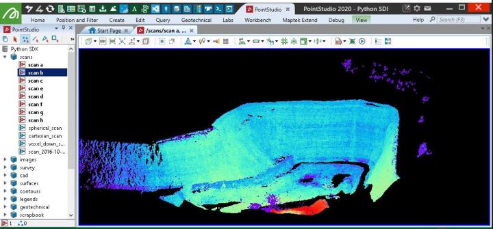
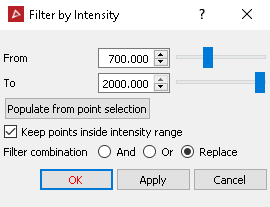
Filtering by intensity
This example shows how to filter data based on intensity ranges within the scan.
import numpy as np
from mapteksdk.project import Project
from mapteksdk.data import Scan

max_intensity = input("Maximum intensity to keep (default = 2000)")
max_intensity = int(max_intensity) if max_intensity.isnumeric() else 2000
min_intensity = input("Minimum intensity to keep (default = 700)")
min_intensity = int(min_intensity) if min_intensity.isnumeric() else 700

proj = Project() # Connect to default project

for item in proj.get_selected():
    # Limit filtering to Scan objects as only they contain the point_intensity attribute
    if item.is_a(Scan):
        with proj.edit(item) as obj:
            if np.any(obj.point_selection):
                # Object has points selected by the user, so only filter out
                # any that are outside the criteria but part of the selection
                selected_and_outside_range = np.where(obj.point_selection
                                                     & ((obj.point_intensity > max_intensity)
                                                       | (obj.point_intensity < min_intensity)))
                obj.point_visibility[selected_and_outside_range] = False
                # As points from the active selection may have been set to hidden,
                # this will remove any that were hidden from the remaining selection.
                # np.logical_not(obj.point_visibility) reverses the booleans so 'invisible == true',
                # and we want to hide where 'invisible == true & selected == true'.
                selected_but_not_visible = np.where(np.logical_not(obj.point_visibility)
                                                      & obj.point_selection)
                obj.point_selection[selected_but_not_visible] = False
            else:
                # No points selected, so apply filter over whole object
                outside_range = np.where((obj.point_intensity > max_intensity)
                                         | (obj.point_intensity < min_intensity))
                obj.point_visibility[outside_range] = False
This will provide similar results to the PointStudio intensity filter tool:
Range filtering
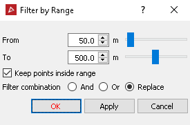
This example shows how to use the range values to filter a scan.
import numpy as np
from mapteksdk.project import Project
from mapteksdk.data import Scan

max_range = input("Maximum range from scanner to keep (default = 500)")
max_range = float(max_range) if max_range.replace(".","").isnumeric() else 500.
min_range = input("Minimum range from scanner to keep (default = 50)")
min_range = float(min_range) if min_range.replace(".","").isnumeric() else 50.

proj = Project() # Connect to default project

for item in proj.get_selected():
    # Limit filtering to Scan objects as only they contain the point_ranges attribute
    if item.is_a(Scan):
        with proj.edit(item) as obj:
            outside_range = np.where((obj.point_ranges > max_range)
                                        | (obj.point_ranges < min_range))
            obj.point_visibility[outside_range] = False
This will provide similar results to the PointStudio range filter tool:
Hiding isolated points over multiple scans
This example uses the open3d library remove_statistical_outlier function to hide isolated points from multiple scans treated as a single combined object.
Note: This example provides a more comprehensive approach to filtering scans, allowing you to run a filter that considers individual scans or multiple scans simultaneously, switching between ‘and’ or ‘replace’ filtering approach and writing the visibility masks back out to individual scans once results are computed. This uses ExitStack from contextlib to allow simultaneous operation on data scopes contained within with context statements. Approaches used here are also useful in point sets (which this snippet will also work with) where you need to filter points while preserving array orders for maintaining integrity on metadata such as attributes.
Note: Most of the code within the main filter function can be used to create new filters with similar requirements for combined-scan operations (see parts surrounding ### Above this line is boilerplate for combined filters ### and ### Below this line is boilerplate for combined filters ###).
Important: This makes use of the open3d library, which is not included by default with Python. You may need to install it before trying the script.
import numpy as np
from mapteksdk.project import Project
from mapteksdk.data import DataObject
from typing import List
from contextlib import ExitStack
import open3d as o3d

def isolated_filter_combined(scans: List[DataObject], nb_neighbors:int=10, std_ratio:float=3, include_hidden:bool=False) -> List[np.array]:
    """Perform an isolated point filter over a collection of Pointsets or Scans treated as a single combined object.
       A list of visibility mask arrays are returned relating to the objects provided.

       This filter combines several objects to filter them as a single entity.
       The computation is performed by the open3d library.

    Args:
        scans (List[DataObject]): List of Scans/Pointsets objects with .points property
        nb_neighbors (int): How many neighbors are taken into account in order to calculate the
                            average distance for a given point.
        std_ratio (float): The threshold level based on the standard deviation of the
                            average distances across the point cloud. The lower this number
                            the more aggressive the filter will be.
        include_hidden (bool, optional): Whether to use indices of existing hidden points in filtered result.
    Returns:
        List[ndarray]: List of arrays of booleans in order of the original objects provided,
                       representing points meeting filter criteria
    """
    # Create array to store all object points, their original point order and object list id
    all_points = np.empty((0,5), dtype=np.float64) # x, y, z, original id, list id
    for i in range(len(scans)):
        scan = scans[i]
        if not all(hasattr(scan, attr) for attr in ["points", "point_visibility", "point_count"]):
            raise Exception(f"Invalid object provided {scan.id.name}. Does not have points.")

        # Create an array to represent original index order and attach it to the point array
        original_indices = np.arange(0, scan.point_count, 1, dtype=np.uint32)
        # Attach id from 'scans' list for putting things back into the right objects at the end
        object_list_id = np.full((scan.point_count), i, dtype=np.uint32)
        # Attach index order and object list id to points array for this object
        points = np.column_stack((scan.points, original_indices, object_list_id))
        # If we don't want to consider already hidden points in the computation, remove them now
        if include_hidden == False:
            points = points[scan.point_visibility]
        # Store points for this object into combined array
        all_points = np.vstack((all_points, points))

    ### Above this line is boilerplate for combined filters ###

    # Actual filter computation:
    # Convert to an open3d point cloud
    pcd = o3d.geometry.PointCloud()
    pcd.points = o3d.utility.Vector3dVector(all_points[:,0:3])
    # Run open3d filter
    cl, ind = pcd.remove_statistical_outlier(nb_neighbors=nb_neighbors, std_ratio=std_ratio)
    # Get list of indices that remain
    vec_int = np.fromiter(ind, dtype = np.int)
    # Apply filter to all_points
    all_points = all_points[vec_int]

    ### Below this line is boilerplate for combined filters ###

    results = []
    # Create filter masks relating to the original objects:
    for i in range(len(scans)):
        # Get points relating to this object only (original list id kept in [:,4], equal to i)
        points_for_this_scan = np.where((all_points[:,4].astype(np.uint32) == i))
        points = all_points[points_for_this_scan]
        # Regenerate original index order then keep matched indices from points above
        original_indices = np.arange(0, scans[i].point_count, 1, dtype=np.uint32)
        # Create array of booleans (visibility mask) on original indicies representing which
        # are still in 'points' after filtering
        results.append(np.isin(original_indices, points[:,3]))
    # Return list of boolean arrays in same order as scans provided to apply masks to scans
    return results

if __name__ == "__main__":
    filter_ratio = input("Enter the threshold level based on the standard deviation of the average distances" \
                        + "across the point cloud.\nThe lower this number the more aggressive the filter will be."
                        + "\n\tDefault = 10.0:\n")
    filter_ratio = float(filter_ratio) if filter_ratio.replace(".","").isnumeric() else 10
    filter_neighbours = input("Enter number of point neighbours taken into account in order to " \
                        +"calculate the average distance for a given point."
                        + "\n\tDefault = 10:\n")
    filter_neighbours = int(filter_neighbours) if filter_neighbours.isnumeric() else 10
    filter_style = input("Use [REPLACE] style or [AND] style filtering?"
                         + "\n\tType: 'replace' (default) or 'and'\n")
    filter_combine = input("Treat all objects as one object for filtering?"
                           + "\n\tType: 'True' (default) or 'False' for filter one-by-one\n")
    filter_combine = False if filter_combine.lower() == "false" else True
    proj = Project() # Connect to default project
    selection = proj.get_selected() # Get the active object selection

    # Use contextlib ExitStack to work with several 'with' contexts simultaneously
    with ExitStack() as stack:
        scans = [stack.enter_context(proj.edit(item)) for item in selection]
        if filter_combine:
            # Run on all objects as as single entity
            try:
               # REPLACE filter (show all, then apply filter) -> filter_style != 'and'
               # AND filter (don't re-show anything already hidden) -> filter_style == 'and'
                results = isolated_filter_combined(scans=scans,
                                                   nb_neighbors=filter_neighbours,
                                                   std_ratio=filter_ratio,
                                                   include_hidden=(filter_style.lower()!="and"))
                for i in range(len(results)):
                    # You can't modify 'scan' points or delete them directly.
                    # Instead we mask/make invisible points to be filtered.
                    scans[i].point_visibility = results[i]
            except Exception as ex:
                print(ex)
        else:
            # Run on each object as individual entities.
            for i in range(len(scans)):
                try:
                    scans[i].point_visibility = isolated_filter_combined(scans=[scans[i]],
                                                                         nb_neighbors=filter_neighbours,
                                                                         std_ratio=filter_ratio,
                                                                         include_hidden=(filter_style.lower()!="and"))
                except Exception as ex:
                    print(ex)
The following animation illustrates the points removed by this filter by re-colouring the scans, then shows the remaining points that were filtered as red.
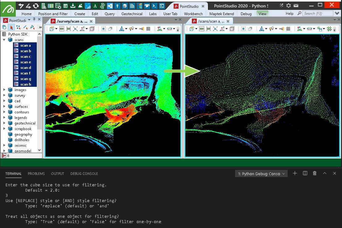
Grid 3D filter over multiple scans
This example applies a 3D filter over equally sized cubes around the data. It is similar to PointStudio's minimum separation filter, but chooses the lowest point within each 3D cube of space. It doesn't guarantee spacing of points will be similar or more than the cell size chosen as two points very close to each other that happen to fall into two grid cells may also be the lowest in the respective grids and be chosen. For a nicer result with more evenly spaced points — see the 'Voxel down sample' example below (however it will create a new object rather than filter existing objects).
Note: This example provides a more comprehensive approach to filtering scans, allowing you to run a filter that considers individual or multiple scans simultaneously, switching between ‘and’ or ‘replace’ filtering approach and writing the visibility masks back out to individual Scan objects once results are computed. This uses ExitStack from contextlib to allow simultaneous operation on data scopes contained within with context statements. Approaches used here are also useful in point sets (which this snippet will also work with) where you need to filter points while preserving array orders for maintaining integrity on metadata such as attributes.
import numpy as np
from mapteksdk.project import Project
from mapteksdk.data import DataObject
from typing import List
from contextlib import ExitStack
import pandas as pd

def grid3d_filter_combined(scans: List[DataObject], cell_size:float=0.1, include_hidden:bool=True) -> List[np.array]:
    """Perform a minimum-separation-like (3d grid) filter over a collection of Pointsets or Scans treated
       as a single combined object. A list of visibility mask arrays are returned relating to the objects provided.

        This filter combines several objects to filter them as a single entity.

        Note: While PointStudio's minimum separation would keep points closest to cube centroids,
        this filter will work more like a 3D topography filter, keeping the lowest point in each cube.

    Args:
        scans (List[DataObject]): List of Scans/Pointsets objects with .points property
        cell_size (float, optional): Filtering size in metres. Defaults to 0.1.
        include_hidden (bool, optional): Whether to use indices of existing hidden points in filtered result.
    Returns:
        List[ndarray]: List of arrays of booleans in order of the original objects provided,
                       representing points meeting filter criteria
    """
    # Create array to store all object points, their original point order and object list id
    all_points = np.empty((0,5), dtype=np.float64) # x, y, z, original id, list id
    for i in range(len(scans)):
        scan = scans[i]
        if not hasattr(scan, 'points') or not hasattr(scan, 'point_visibility') or not hasattr(scan, 'point_count'):
            raise Exception(f"Invalid object provided {scan.id.name}. Does not have points.")

        # Create an array to represent original index order and attach it to the point array
        original_indices = np.arange(0, scan.point_count, 1, dtype=np.uint32)
        # Attach id from 'scans' list for putting things back into the right objects at the end
        object_list_id = np.full((scan.point_count), i, dtype=np.uint32)
        # Attach index order and object list id to points array for this object
        points = np.column_stack((scan.points, original_indices, object_list_id))
        # If we don't want to consider already hidden points in the computation, remove them now
        if include_hidden == False:
            points = points[scan.point_visibility]
        # Store points for this object into combined array
        all_points = np.vstack((all_points, points))

    # For filtering performance, sort the point data by height (across all objects)
    # (we need to un-sort later, hence attaching original_indices to the array in [:,3])
    sorted_indices = all_points[:, 2].argsort() # [:, 2] = sort by z
    # Re-order the array to z-sorted order
    all_points = all_points[sorted_indices]

    # Create a grid around the data by snapping X and Y values into grid.
    # This is most conveniently done in Pandas.
    filter_pts = pd.DataFrame(all_points[:, 0:3], columns=['X', 'Y', 'Z'])
    # Snap all points to consistent x/y grid
    filter_pts["X_Grid"] = np.round(filter_pts['X']/cell_size)*cell_size
    filter_pts["Y_Grid"] = np.round(filter_pts['Y']/cell_size)*cell_size
    filter_pts["Z_Grid"] = np.round(filter_pts['Z']/cell_size)*cell_size

    # head(1) = keep 1st in group (i.e. lowest)
    filtered_indices = filter_pts.groupby(['X_Grid', 'Y_Grid', 'Z_Grid'])['Z'].head(1).index

    # Reset point array to be the filtered points
    keep_indices = np.isin(filter_pts.index, filtered_indices)

    results = []
    # Create filter masks relating to the original objects:
    for i in range(len(scans)):
        # Filter points to indices to keep
        points = all_points[keep_indices]
        # Get points relating to this object only (original list id kept in [:,4], equal to i)
        points_for_this_scan = np.where((points[:,4].astype(np.uint32) == i))
        points = points[points_for_this_scan]
        # Restore array order to match original point order (original point ids in [:,3])
        points = points[points[:,3].argsort()]
        # Regenerate original index order then keep matched indices from points above
        original_indices = np.arange(0, scans[i].point_count, 1, dtype=np.uint32)
        # Create array of booleans (visibility mask) on original indices representing which
        # are still in 'points' after filtering
        results.append(np.isin(original_indices, points[:,3]))
    # Return list of boolean arrays in same order as scans provided to apply masks to scans
    return results

if __name__ == "__main__":
    filter_size = input("Enter the cube size to use for filtering.\n\tDefault = 2.0:\n")
    filter_size = float(filter_size) if filter_size.replace(".","").isnumeric() else 2.0
    filter_style = input("Use [REPLACE] style or [AND] style filtering?"
                         + "\n\tType: 'replace' (default) or 'and'\n")
    filter_combine = input("Treat all objects as one object for filtering?"
                           + "\n\tType: 'True' (default) or 'False' for filter one-by-one\n")
    filter_combine = False if filter_combine.lower() == "false" else True
    proj = Project() # Connect to default project
    selection = proj.get_selected()

    # Use contextlib ExitStack to work with several 'with' contexts simultaneously
    with ExitStack() as stack:
        scans = [stack.enter_context(proj.edit(item)) for item in selection]
        if filter_combine:
            # Run on all objects as as single entity
            try:
                # REPLACE filter (show all, then apply filter) -> filter_style != 'and'
                # AND filter (don't re-show anything already hidden) -> filter_style == 'and'
                results = grid3d_filter_combined(
                    scans=scans,
                    cell_size=filter_size,
                    include_hidden=(filter_style.lower()!="and"))
                for i in range(len(results)):
                    # You can't modify 'scan' points or delete them directly.
                    # Instead we mask/make invisible points to be filtered.
                    scans[i].point_visibility = results[i]
            except Exception as ex:
                print(ex)
        else:
            # Run on each object as individual entities.
            for i in range(len(scans)):
                try:
                    results = grid3d_filter_combined(
                        scans=[scans[i]],
                        cell_size=filter_size,
                        include_hidden=(filter_style.lower()!="and"))
                except Exception as ex:
                    print(ex)
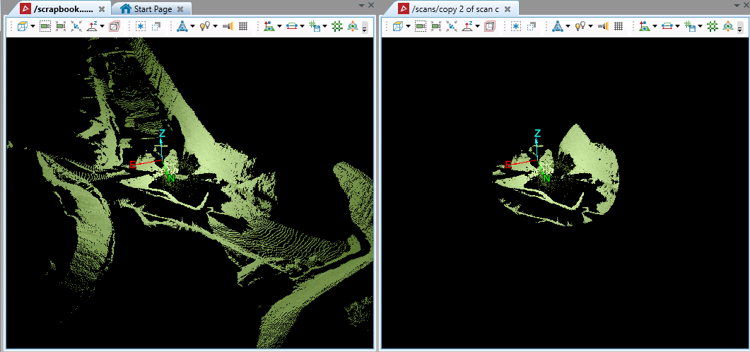
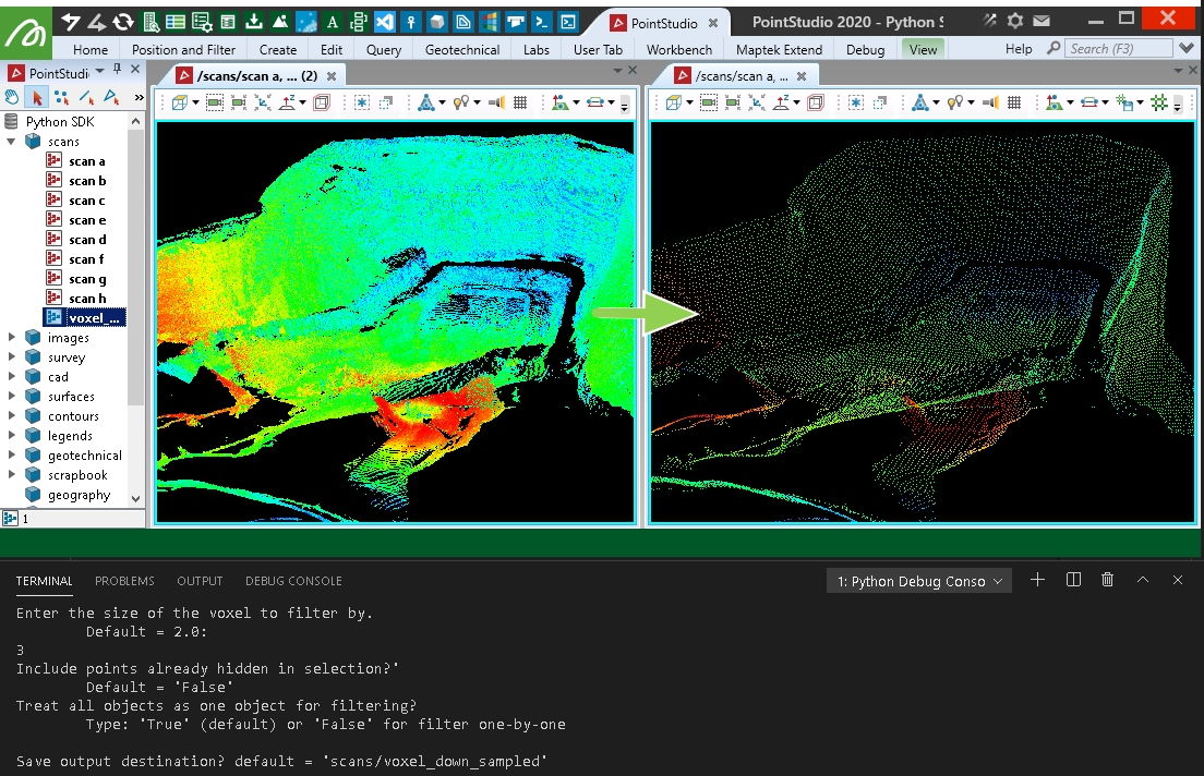
Creating an even spread of points using voxel down-sample
This example will take points from a collection of scans and use the open3d voxel_down_sample function to create a new object with points that are nicely spread and spaced by a range of 3D voxels over the data.
Important: This makes use of the open3d library, which is not included by default with Python. You may need to install it before trying the script.
import numpy as np
from mapteksdk.project import Project
from mapteksdk.data import DataObject, Scan
from typing import List, Tuple
from contextlib import ExitStack
import open3d as o3d

def voxel_down_sample(scans: List[DataObject], voxel_size:float=1., include_hidden:bool=False)-> Tuple[np.array, np.array]:
    """Uses the open3d library to create a sub-sampled scan using Voxels.

       All input data will be combined into a single entity to do this.

    Args:
        scans (List[DataObject]): List of Scans/Pointsets
                                  objects with .points property
        voxel_size (float): Filter size in metres
        include_hidden (bool, optional): Whether to use indices of existing
                                         hidden points in filtered result.
    Returns:
        Tuple(ndarray(points), ndarray(colours))
    """
    # Create array to store all object points, their original point order and object list id
    all_points = np.empty((0,3), dtype=np.float64) # x, y, z
    all_colours = np.empty((0,3), dtype=np.uint8) # r, g, b
    for i in range(len(scans)):
        scan = scans[i]
        if not all(hasattr(scan, attr) for attr in ["points", "point_colours", "point_count"]):
            raise Exception(f"Invalid object provided {scan.id.name}. Does not have points.")

        # Attach index order and object list id to points array for this object
        points, colours = scan.points, scan.point_colours[:, 0:3] # Get R,G,B, not R,G,B,A
        # If we don't want to consider already hidden points in the computation, remove them now
        if include_hidden == False:
            points = points[scan.point_visibility]
            colours = colours[scan.point_visibility]
        # Store points for this object into combined array
        all_points = np.vstack((all_points, points))
        all_colours = np.vstack((all_colours, colours))

    # Actual filter computation:
    # Convert to an open3d point cloud
    pcd = o3d.geometry.PointCloud()
    pcd.points = o3d.utility.Vector3dVector(all_points)
    # o3d uses RGB ranges between 0-1 (need to convert from 0-255)
    all_colours = all_colours.astype(np.float64) / 255.0
    pcd.colors = o3d.utility.Vector3dVector(all_colours)
    # Run open3d filter
    pcd = pcd.voxel_down_sample(voxel_size=voxel_size)
    # Convert back to numpy arrays we can use
    all_points = np.asarray(pcd.points)
    all_colours = (np.asarray(pcd.colors) * 255).astype(np.uint8)
    # add alpha column onto colours
    alpha = np.full((all_colours.shape[0], 1), 255, dtype=np.uint8)

    all_colours = np.column_stack((all_colours, alpha))

    return (all_points, all_colours)

if __name__ == "__main__":
    filter_size = input("Enter the size of the voxel to filter by.\n\tDefault = 2.0:\n")
    filter_size = float(filter_size) if filter_size.replace(".","").isnumeric() else 2.0
    filter_style = input("Include points already hidden in selection?'\n\tDefault = 'False'")
    filter_style = True if filter_style.lower() == "true" else False
    filter_combine = input("Treat all objects as one object for filtering?"
                           + "\n\tType: 'True' (default) or 'False' for filter one-by-one\n")
    filter_combine = False if filter_combine.lower() == "false" else True
    save_path = input("Save output destination? default = 'scans/voxel_down_sampled'\n")
    save_path = "scans/voxel_down_sampled" if len(save_path) == 0 else save_path
    proj = Project() # Connect to default project
    selection = proj.get_selected()

    # Use contextlib ExitStack to work with several 'with' contexts simultaneously
    with ExitStack() as stack:
        scans = [stack.enter_context(proj.edit(item)) for item in selection]
        if filter_combine:
            # Run on all objects as as single entity
            with proj.new(save_path, Scan, overwrite=True) as new_scan:
                new_scan.points, new_scan.point_colours = voxel_down_sample(scans=scans,
                                                                            voxel_size=filter_size,
                                                                            include_hidden=filter_style)
        else:
            # Run on each object as individual entities.
            for i in range(len(scans)):
                with proj.new(f"{save_path} of {scans[i].id.name}", Scan, overwrite=True) as new_scan:
                    new_scan.points, new_scan.point_colours = voxel_down_sample(scans=[scans[i]],
                                                                                voxel_size=filter_size,
                                                                                include_hidden=filter_style)
Applying a topographic filter
This example does a 2D filter over equally sized grid cells around the data. It is similar to PointStudio's topography filter, with options to choose the highest or lowest falling in each cell as well as treating all scans as a single object for the filter process. It doesn't guarantee spacing of points will be similar or more than the cell size chosen as two points very close to each other that happen to fall into two grid cells may also be the lowest in the respective grids and be chosen.
A basic approach to this same filter is also provided in the examples described in Point Sets.
Note: This example provides a more comprehensive approach to filtering scans, allowing you to run a filter that considers individual scans or multiple scans simultaneously, switching between ‘and’ or ‘replace’ filtering approach and writing the visibility masks back out to individual scans once results are computed. This uses ExitStack from contextlib to allow simultaneous operation on data scopes contained within with context statements. Approaches used here are also useful in point sets (which this snippet will also work with) where you need to filter points while preserving array orders for maintaining integrity on metadata such as attributes.
import numpy as np
import pandas as pd
from mapteksdk.project import Project
from mapteksdk.data import DataObject
from typing import List
from contextlib import ExitStack

def topography_filter_single(scan: DataObject, cell_size:float=0.1, keep_lowest:bool=True, include_hidden:bool=True) -> np.array:
    """Perform a topography (grid) filter over a single Pointset or Scan.
        A visibility mask array is returned.

    Args:
        scan (Scan or PointSet): Scan or Pointset object with .points property
        cell_size (float, optional): Filtering size in metres. Defaults to 0.1.
        keep_lowest (bool, optional): True=Keep Lowest, False=Keep Highest. Defaults to True.
        include_hidden (bool, optional): Whether to use indices of existing hidden points in filtered result.
    Returns:
        ndarray: Array of booleans representing points meeting filter criteria
    """
    if not hasattr(scan, 'points') or not hasattr(scan, 'point_visibility'):
        raise Exception(f"Invalid object provided {scan.id.name}. Does not have points.")
    # Create an array to represent original index order and attach it to the point array
    original_indices = np.arange(0, scan.point_count, 1, dtype=np.uint32)
    points = np.column_stack((scan.points, original_indices))
    # If we don't want to consider already hidden points in the computation, remove them now
    if include_hidden == False:
        points = points[scan.point_visibility]
    # For filtering performance, sort the point data by height (we need to un-sort later)
    sorted_indices = points[:, 2].argsort() # sort by z
    points = points[sorted_indices]

    #intensities = intensities[sorted_indices] if intensities is not None else None
    # Create a grid around the data by snapping X and Y values into grid
    filter_pts = pd.DataFrame(points, columns=['X', 'Y', 'Z', 'original_id'])
    filter_pts["X_Grid"] = np.round(filter_pts['X']/cell_size)*cell_size
    filter_pts["Y_Grid"] = np.round(filter_pts['Y']/cell_size)*cell_size
    if keep_lowest:
        # head(1) = keep 1st in group (i.e. lowest)
        filtered_indices = filter_pts.groupby(['X_Grid', 'Y_Grid'])['Z'].head(1).index
    else:
        # tail(1) = last 1st in group (i.e. highest)
        filtered_indices = filter_pts.groupby(['X_Grid', 'Y_Grid'])['Z'].tail(1).index
    # Reset point array to be the filtered points
    keep_indices = np.isin(filter_pts.index, filtered_indices)
    # Filter points to indices to keep
    points = points[keep_indices]
    # Restore array order to match original point order
    points = points[points[:,3].argsort()]
    # Return booleans on original indicies representing which are still in 'points' after filtering
    return np.isin(original_indices, points[:,3])

def topography_filter_combined(scans: List[DataObject], cell_size:float=0.1, keep_lowest:bool=True, include_hidden:bool=True) -> List[np.array]:
    """Perform a topography (grid) filter over a collection of Pointsets or
        Scans treated as a single combined object.
        A list of visibility mask arrays are returned relating to the objects provided.

        This filter combines several objects to filter them as a single entity.

    Args:
        scans (List[DataObject]): List of Scans/Pointsets objects with .points property
        cell_size (float, optional): Filtering size in metres. Defaults to 0.1.
        keep_lowest (bool, optional): True=Keep Lowest, False=Keep Highest. Defaults to True.
        include_hidden (bool, optional): Whether to use indices of existing hidden points in filtered result.
    Returns:
        List[ndarray]: List of arrays of booleans in order of the original objects provided,
                       representing points meeting filter criteria
    """
    # Create array to store all object points, their original point order and object list id
    all_points = np.empty((0,5), dtype=np.float64) # x, y, z, original id, list id
    for i in range(len(scans)):
        scan = scans[i]
        if not all(hasattr(scan, attr) for attr in ["points", "point_visibility", "point_count"]):
            raise Exception(f"Invalid object provided {scan.id.name}. Does not have points.")

        # Create an array to represent original index order and attach it to the point array
        original_indices = np.arange(0, scan.point_count, 1, dtype=np.uint32)
        # Attach id from 'scans' list for putting things back into the right objects at the end
        object_list_id = np.full((scan.point_count), i, dtype=np.uint32)
        # Attach index order and object list id to points array for this object
        points = np.column_stack((scan.points, original_indices, object_list_id))
        # If we don't want to consider already hidden points in the computation, remove them now
        if include_hidden == False:
            points = points[scan.point_visibility]
        # Store points for this object into combined array
        all_points = np.vstack((all_points, points))

    # For filtering performance, sort the point data by height (across all objects)
    # (we need to un-sort later, hence attaching original_indices to the array in [:,3])
    sorted_indices = all_points[:, 2].argsort() # [:, 2] = sort by z
    # Re-order the array to z-sorted order
    all_points = all_points[sorted_indices]

    # Create a grid around the data by snapping X and Y values into grid.
    # This is most conveniently done in Pandas.
    filter_pts = pd.DataFrame(all_points[:, 0:3], columns=['X', 'Y', 'Z'])
    # Snap all points to consistent x/y grid
    filter_pts["X_Grid"] = np.round(filter_pts['X']/cell_size)*cell_size
    filter_pts["Y_Grid"] = np.round(filter_pts['Y']/cell_size)*cell_size
    if keep_lowest:
        # head(1) = keep 1st in group (i.e. lowest)
        filtered_indices = filter_pts.groupby(['X_Grid', 'Y_Grid'])['Z'].head(1).index
        # If you wanted to keep more than '_the_ lowest point' - increase .head(1).
    else:
        # tail(1) = last 1st in group (i.e. highest)
        filtered_indices = filter_pts.groupby(['X_Grid', 'Y_Grid'])['Z'].tail(1).index
        # If you wanted to keep more than '_the_ highest point' - increase .tail(1).

    # Reset point array to be the filtered points
    keep_indices = np.isin(filter_pts.index, filtered_indices)

    results = []
    # Create filter masks relating to the original objects:
    for i in range(len(scans)):
        # Filter points to indices to keep
        points = all_points[keep_indices]
        # Get points relating to this object only (original list id kept in [:,4], equal to i)
        points_for_this_scan = np.where((points[:,4].astype(np.uint32) == i))
        points = points[points_for_this_scan]
        # Restore array order to match original point order (original point ids in [:,3])
        points = points[points[:,3].argsort()]
        # Regenerate original index order then keep matched indices from points above
        original_indices = np.arange(0, scans[i].point_count, 1, dtype=np.uint32)
        # Create array of booleans (visibility mask) on original indicies representing which
        # are still in 'points' after filtering
        results.append(np.isin(original_indices, points[:,3]))
    # Return list of boolean arrays in same order as scans provided to apply masks to scans
    return results

if __name__ == "__main__":
    filter_size = input("Enter filter size (m) - default = 1.0:\n") # 1m cells
    filter_size = float(filter_size) if filter_size.replace(".","").isnumeric() else 1.0
    filter_style = input("Use [REPLACE] style or [AND] style filtering?"
                         + "\n\tType: 'replace' (default) or 'and'\n")
    filter_combine = input("Treat all objects as one object for filtering?"
                           + "\n\tType: 'True' (default) or 'False' for filter one-by-one\n")
    filter_combine = False if filter_combine.lower() == "false" else True
    filter_lowest = input("Keep Lowest ('True'/Default) or Highest('False')?\n")
    filter_lowest = False if filter_lowest.lower() == "false" else True
    proj = Project() # Connect to default project
    selection = proj.get_selected()

    # Use contextlib ExitStack to work with several 'with' contexts simultaneously
    with ExitStack() as stack:
        scans = [stack.enter_context(proj.edit(item)) for item in selection]
        if filter_combine:
            # Run on all objects as as single entity
            try:
               # REPLACE filter (show all, then apply filter) -> filter_style != 'and'
               # AND filter (don't re-show anything already hidden) -> filter_style == 'and'
               results = topography_filter_combined(scans=scans,
                                                    cell_size=filter_size,
                                                    include_hidden=(filter_style.lower()!="and"),
                                                    keep_lowest=filter_lowest)
               for i in range(len(results)):
                    # You can't modify 'scan' points or delete them directly.
                    # Instead we mask/make invisible points to be filtered.
                    scans[i].point_visibility = results[i]
            except Exception as ex:
                print(ex)
        else:
            # Run on each object as individual entities.
            # You can use topography_filter_combined with a single object in the list,
            # however topography_filter_single is used here for demonstration.
            for i in range(len(scans)):
                try:
                    scans[i].point_visibility = topography_filter_single(scan=scans[i],
                                                                         cell_size=filter_size,
                                                                         include_hidden=(filter_style.lower()!="and"),
                                                                         keep_lowest=filter_lowest)
                except Exception as ex:
                    print(ex)