Creating a Cross Variogram

This option studies the effect one element has on another.

Click for tutorial: Chart Viewing and Exporting

Note: The Properties panel for Cross Variograms is like that of the Semivariogram. However, two variables are needed instead of one in order to generate the experimental cross variograms.

On the Variography tab, in the Charts group, click Cross Variogram.

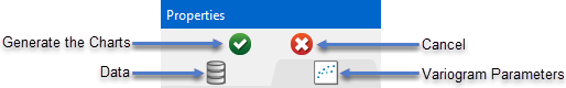
When you click Cross Variogram in the ribbon, the Properties panel on the right will populate with various options.

Axis Settings

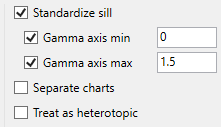
Standardise Sill

Select this check box if you want to standardise the variogram sill by dividing the results by the sample variance. This is useful when calculating a semivariogram because instead of reaching the sill at the sample variance it will reach it at 1.

Gamma axis min / max (Optional)

Select one or both of these options if you want to set the minimum or maximum extents of the gamma axis.

Separate Charts

Select this option to display separate charts for each set of variogram parameters.

Treat as heterotopic

Since a cross variogram measures the difference between two variables at a given location, a problem arises when the locations of sample points between the two datasets are different. Select this option to perform heterotopic cokriging when you are working with unequally sampled data and multiple databases.

Omni-Directional

An omnidirectional variogram considers all directions in the same calculation. It can be thought of as an average variogram of multiple directional variograms. However, it doesn't mean that the spatial continuity is equal in every direction.

Omnidirectional variograms are a good starting point when trying to look for the structure of the overall continuity of a domain.

Down Hole

It is common practice to calculate a down hole variogram to acquire a nugget, and then use that nugget value while calculating a standard variogram.

Depth field

Set this to reflect which variable in the dataset corresponds to the depth field.

Single Direction

By default, this option will be selected. This is the standard option to create an experimental semivariogram.

Directional Properties

Search radius

The search radius should correspond to approximately half the distance of your data field. if the search radius is greater than the halfway point, then the search will over-extend the edge of the data.

Example: If the distance traversing your sample area is 500 feet, then set the search radius to 250 feet.

Lag size

The lag size is the distance for each step from the origin. Set a lag size that coincides with your data spacing.

Example: If your samples are spaced 50 feet apart, then set your lag size to 50. If you have to err, do so on the side of too small.

Lag tolerance

The lag tolerance is the distance plus or minus the lag size that samples will be captured. This helps capture samples that are not located at the exact distance interval as the lag spacing. Set the distance within which to use samples.

Note: If this is set to 0, then the tolerance is not used.

Samples are rarely located at exact intervals such as every 50 feet throughout the entire domain. There will nearly always be some variance. You can capture the samples that are not at exact intervals by setting the variogram to recognise samples that fall within 25 feet of the lag size, which in our sample case is every 50 feet.

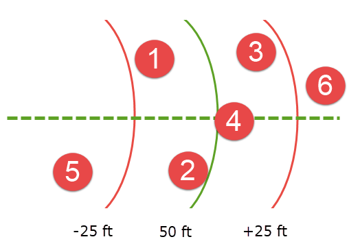
Here, the green line represents a lag size of 50 feet, and the red lines represent a lag tolerance of 25 feet on either side. Samples 1, 2, 3, and 4 would be used in the calculation. However, samples 5 and 6 would be ignored.

Lag tolerance ratio

This corresponds to the percentage of the lag size that is used by the lag tolerance.

Example: A lag size of 50 with a lag tolerance of 25 will result in a lag tolerance ratio of 50%.

Azimuth

Enter the azimuth. This parameter controls the azimuth direction in which variography is evaluated.

Plunge

Enter the plunge. This parameter controls the plunge direction in which variography is evaluated.

Tolerance thresholds

Collectively, the azimuth tolerance, plunge tolerance, horizontal tolerance, and vertical tolerance are known as the Cone of Tolerance. Using too large of a cone can result in excessive mixing of samples from different directions. This can cause the apparent anisotropy to appear smaller than the true anisotropy. Using too small a cone can result in rough variograms that are hard to interpret. The sample cone may be too small if the number of sample pairs for most lags is small compared to the number of sample points.

For an omnidirectional variogram, use 90 for the azimuth tolerance and 90 for the cone angle tolerance.

Note: At a great enough distance, the horizontal distance tolerance and vertical distance tolerance will clip the sides of the search cone.

Azimuth tolerance

Enter the limit on the angle between two samples as measured in the plane of the plunge of the variogram.

Plunge tolerance

Enter the limit on the angle between two samples as measured in a vertical plane in the direction of the azimuth.

Note: A combination of cone, azimuth and plunge tolerances is used if the azimuth angle tolerance and plunge angle tolerance are set to less than the cone angle tolerance.

Horizontal tolerance

Enter the horizontal distance limit on sample pairs. Any acceptable sample must be within this horizontal distance of the centre of the variogram cone.

Tip: Set this value to a typical spacing (or larger) between your data, for example, if your data is on a 100 × 100 × 10 grid, set a horizontal distance of 100 and a vertical tolerance of 10. If you receive too few sample pairs, try increasing the tolerances to capture more data otherwise artifacts such as "hole effects" may occur.

Vertical tolerance

Enter the vertical distance limit on sample pairs. Any acceptable sample must be within this vertical distance from the centre of the variogram cone. The vertical distance is measured from the plane of the plunge of the variogram cone.

Multiple Directions

Unfolding

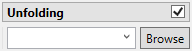
The unfolding option is used in the case of deformed strata bound deposits. This can be applied to deposits where mineralisation is controlled by a structural surface that can be modelled. The specification file from a Grid Model is used.

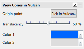
View Cones in Vulcan

You can visualise the search ellipses by enabling the option to View Cones in Vulcan, or by clicking Display Cones from the Connectivity tab in the ribbon. The cones are interactive, therefore, any changes made in the variogram parameters will be automatically reflected in the cones seen in Vulcan.

Steps

Begin by clicking the button labelled Pick in Vulcan.
In the Envisage workspace, click where you want the origin of the cones to be displayed.
Use the slider to adjust the Translucency of the cones.
Set the colours for the cone by clicking on Colour 1 and Colour 2, then selecting a colour from the palette.
To remove a the cone from the screen, disable the View Cones in Vulcan checkbox.

Note

After you have set the parameters for a cone, it can be displayed using the icons found on the Connectivity tab on the ribbon.

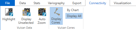
Click Display Cones, then select either By Chart or Display All.

By Chart - Only the charts that have the View Cones in Vulcan option enabled will be displayed.

Display All - All cones will be displayed regardless of whether or not the View Cones in Vulcan option has been enabled.