Univariate Estimation Editor
Use the Univariate Estimation Editor option to perform grade estimations on your block model. The Univariate Estimation Editor allows you to set up parameters used to perform inverse distance, simple kriging, ordinary kriging, indicator kriging, and uniform conditioning for a single variable.
Note: To set up parameters to perform calculations for multiple variables, use the Multivariate Estimation Editor instead. Use the Validation Editor to perform Jack Knife and Cross Validation.
Instructions
On the Block menu, point to Grade Estimation, then click Univariate Estimation Editor.
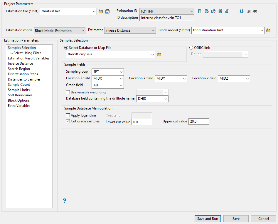
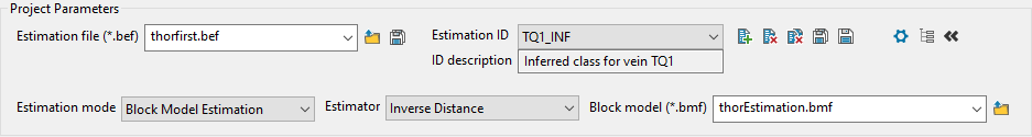
Samples Selection
Follow these steps:
-
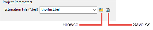
Enter a name for the Estimation file, or select it from the drop-down list. The drop-down list displays all files found in the current working directory that have the (.bef) extension. Click Browse to select a file from another location.
Note: The information entered here is also used to provide the name of the report that is generated and stored in your project folder. The naming convention used for the report is
<bef_file>_<estimation id>.bef_report. The reports can be opened with Vulcan"s Text Editor, or any other text editor.TipYou can make changes to an existing estimation file, then click the Save As icon to save the edited version under a new name. This allows you to transfer all the parameter settings from the Estimation Editor to the new file without having to enter everything in again.
-
Enter or select an Estimation ID. To create a new estimation ID, click the New icon as shown below, and provide a unique name for the current panel settings. Up to nine separate IDs can be created for each BEF file.
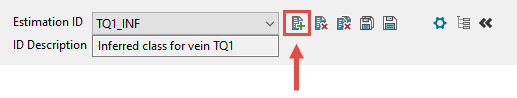
Figure 1 : Click to create a new estimation ID.
The ID Description is optional and is not required. However, they can be very helpful, especially when you are creating multiple IDs.
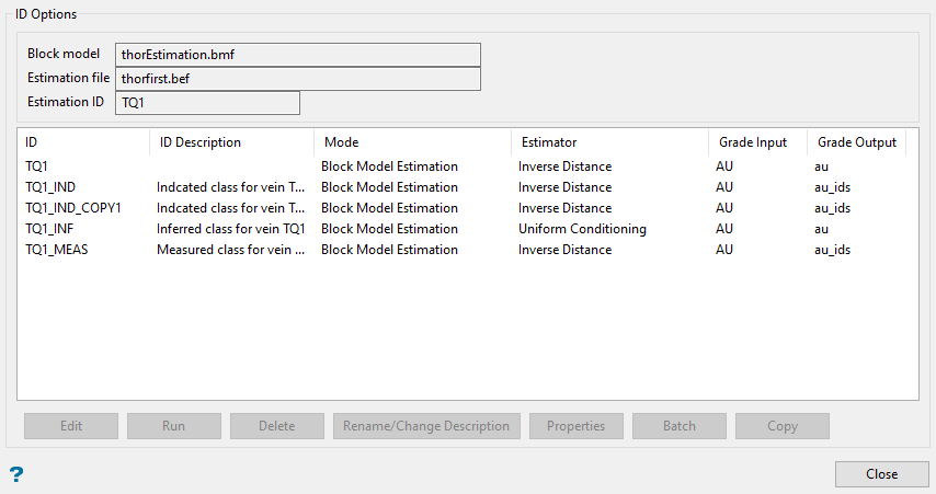
If you need to edit these fields you may do so by clicking the icon to open the estimation file Options panel, then make your changes.
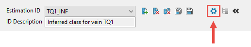
Figure 2 : Click to open the estimation file Options panel.
 ID Options
-
Run - Select this option to perform an estimation using the highlighted estimation ID. This option can only be used to perform a single estimation run. As a result, this option will be unavailable when multiple IDs have been highlighted. If you want to run multiple estimation jobs, use the Batch option instead.
-
Delete - Select this option to delete the highlighted estimation ID. Once selected, you will need to confirm the deletion before the estimation parameters are removed from the associated block estimation file.
-
Rename/Change Description - Select this option to rename the highlighted estimation ID. Once selected, the Rename estimation panel displays. Enter the new estimation ID. Select OK to assign the new estimation ID.
-
Properties - Select this option to display the estimation parameters for the highlighted estimation ID. Once selected, a properties window displays.
-
Batch - Select this option to run multiple estimation jobs using the highlighted estimation IDs. Once selected, the Batch panel displays.
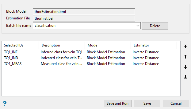
The estimations will be run in the order that they appear in the list. You can edit the order by highlighting an ID, then clicking the arrows on the right side of the panel.
Entering a Batch file name will enable the Save and Run button.
-
Copy - Select this option to copy the highlighted estimation ID. The '_COPY1' value will be appended to the end of the copied estimation ID, as shown in the Estimation ID Options panel above.
Setting up multiple estimation passes
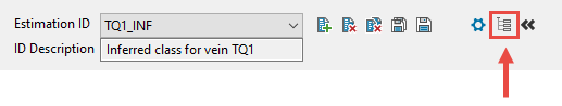
Click the Estimation Passes icon located at the top of the panel, as shown below.
Tip: This should be done after you have completed the main panel entries for the initial estimation pass.
Passes Configuration panel
Click the Estimation Passes icon located at the top of the panel, as shown below.
Tip: This should be done after you have completed the main panel entries for the initial estimation pass.
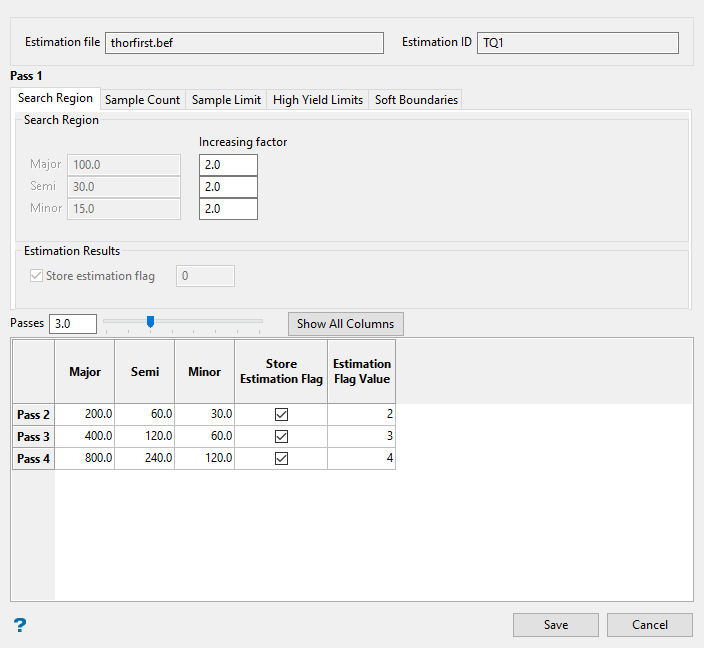
Figure 3 : Estimation Editor Passes Configuration panel.
The Passes Configuration panel uses tabs that divide the input sections into five separate areas: Search Region, Sample Count, Sample Limit, High Yield Limits, and Soft Boundaries. However, you can view all of the input sections as one large table by clicking the Show All Columns button.
Note: The greyed-out fields show the values in place from the main panel. These cannot be edited.
In Search Region, you can either set an Increasing Factor to automatically calculate a new value for each successive pass, or type a value directly into the table cells.
Example: A value of 2 will increase each successive pass by a factor of 2. If the initial pass has a Major value of 100, then the second pass will have a value of 200, the third pass will have a value of 400, the fourth pass will have a value of 800, etc.
Enter the number of passes you want by typing into the Passes field, or by using the slider.
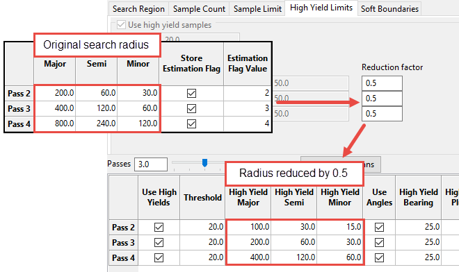
In High Yield Limits, enter a Reduction Factor between 0 and 1. This represents the percentage that the search radius will be reduced.
-
-
-
Select the Estimation Mode from the options in the drop-down list. There are three options available.
-
Block Model Estimation - Perform standard estimation using non-declustered data and customised distances to samples. This is the most common type of estimation. The estimators available when using this option are inverse distance, simple kriging, ordinary kriging, indicator kriging, and uniform conditioning.
-
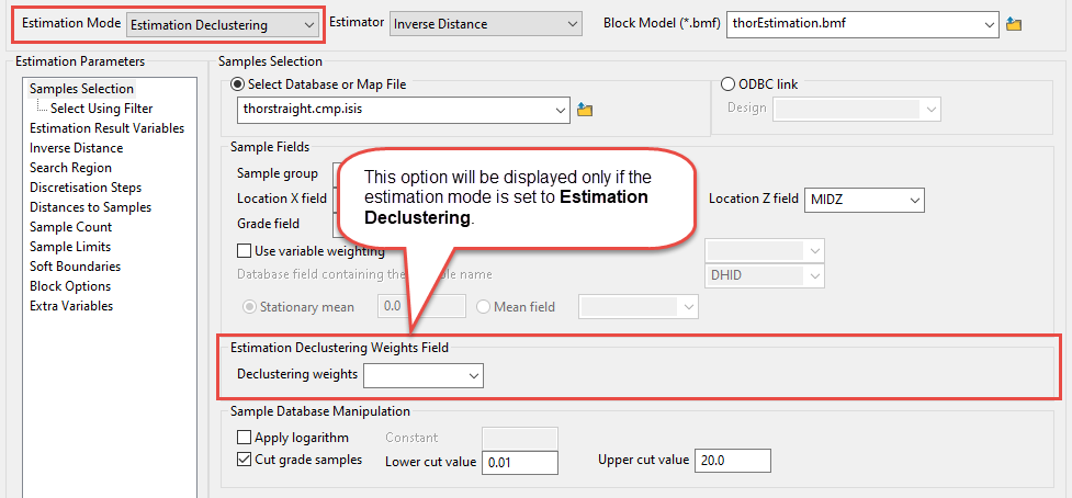
Estimation Declustering - Use declustered data while estimating. The estimators available when using this option are inverse distance, simple kriging, and ordinary kriging
NoteUsing this option will require you to select a declustering weight variable from the block model. If your block model does not have a declustering weight variable, you will not be able to use this option.
-
Global Estimation - Perform estimation using non-declustered data and without limitations applied to search distances. The estimators available when using this option are simple kriging and ordinary kriging.
-
Select the type of Estimator you want to apply. The options will change depending on your selection of estimator.
-
Select the Block Model from the drop-down list. The drop-down list displays all files found in the current working directory that have the (.bmf) extension. Click Browse to select a file from another location.
-
Specify the name of the database or mapfile that contains the sample data. The drop-down list labelled Select Database or Map File contains all of the Vulcan database files and mapfiles found within your current working directory. Click Browse to select a file from another location.
Alternatively, you can use an ODBC link to connect to a database that contains the sample data. Click here for information about ODBC databases.
-
Enter the name of the Sample Group (database key) to be loaded. Wildcards (* multi-character wildcard and % single character wildcard) may be used to select multiple groups.
Note: Multiple groups only apply to Isis databases (ASCII mapfiles consist of one group).
-
Select the names of the fields containing the X, Y and Z coordinates from the Location field drop-down lists.
-
Select the field that the estimates will be calculated from using the Grade field drop-down list.
-
Select the Use variable weighting checkbox if you want to multiply the sample weights by the value of the specified weighting variable. The weighting variable may represent a specific gravity, sample length, or sample weight.
A block with two samples is to be estimated. The first sample has a grade value of
2and a weight variable of1.The second sample has a grade value of5and a weight variable of2.5.The weights, from ordinary kriging, are 0.8 for the first sample and 0.2 for the second sample. Without variable weighting the estimated grade is:(0.8 × 2 + 0.2 × 5) = 2.6With variable weighting the estimate is:
(0.8 × 1 × 2 + 0.2 × 2.5 × 5) ÷ ( 0.8 × 1 + 0.2 × 2.5 ) = 3.15385If the variable weighting is
0for a block, then the default grade value is stored. -
In the section labelled Sample Database Manipulation you can apply the base logarithm function to all sample values. Click Apply logarithm, and then enter the constant that you want to use.
Note: All original sample values must be positive for the logarithm to be defined.
The specified logarithm constant is added to the calculated logarithm.
-
If you want to apply cut-offs to the grades used in the estimation, click Use cut grades. Specify a lower grade cut value (grades lower than this value are set to this value) and an upper grade cut value (grades above this value are set to this value).
Select Using Filter
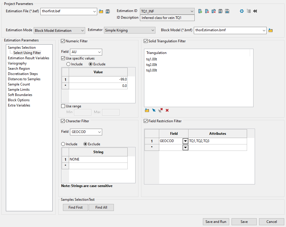
Use this panel to filter your sample data by setting restrictions on samples values, triangulations used, character values within database fields, and field attributes. You can use any combination of the four filters, or not use any at all. This panel is optional.
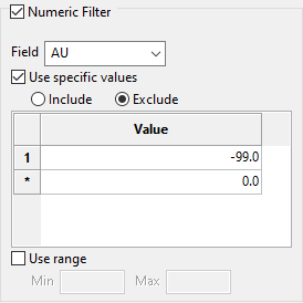
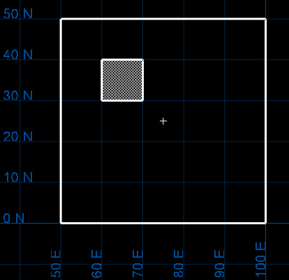
Example: The example above shows one possible way to filter data. The filters will ignore all default assay values of -99.0, include only samples that fall within the three vein triangulations, ignore any sample that has a GEOCOD string equal to "NONE", and include samples that have an attribute label of TQ1, TQ2, or TQ3.
The following steps show how to set your filters.
-
Select the Numeric Filter checkbox to apply numeric restrictions to any field you select from the Field drop-down list. You can use specific values, a range of values, or both.
Note: Only numeric fields will be shown in the drop-down list.
-
Select the option Use specific values to include or exclude whatever values you list under Values in the grid.
-
To use a range of values, select Use range, then enter the minimum and maximum values.
The range below is evaluated as
0.001 ≤ VALUE < 99999.0.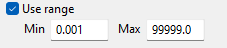
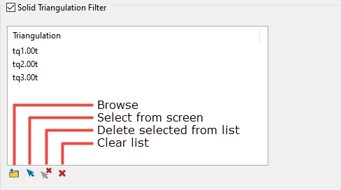
Select the Solid Triangulation Filter checkbox to limit the data by triangulation.
-
Clicking the Browse icon will display the following panel. From here you can select your triangulations. All triangulations found in the current working directory will be listed in the selection panel that will be displayed.
-
Selecting images from the panel
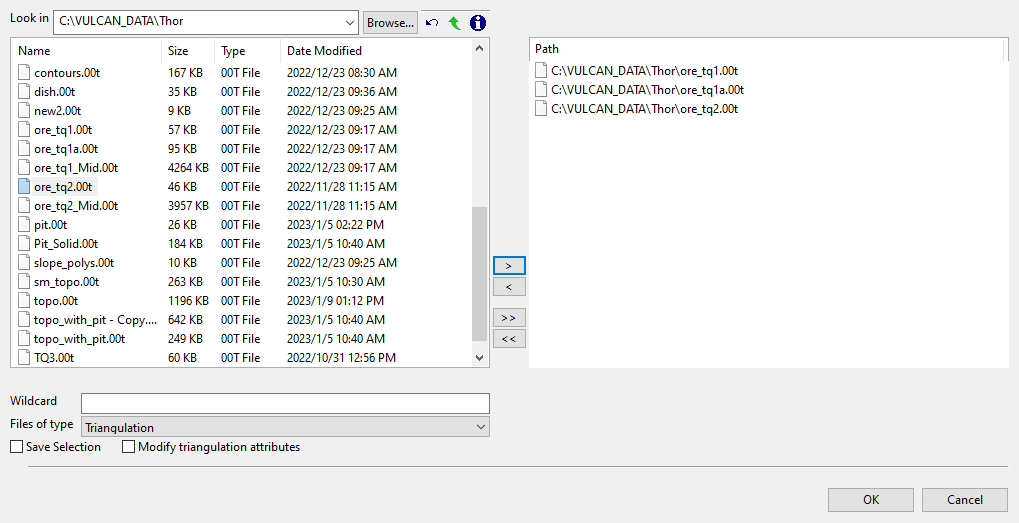
Click the Browse button to search for any triangulation not found in your current working directory.
Click on the name of the file(s) you want to select. Use the
 icons to go to the last folder visited, go up one level, or change the way details are viewed in the window.
To highlight multiple files that are adjacent to each other in the list, hold down the Shift key and click the first and last file names in that section of the list.
To highlight multiple non-adjacent files, hold down the CTRL key while you click the file names.
Move the items to the selection list on the right side of the panel.
- Click the
 button to move the highlighted items to the selection list on the right.
 - Click the
 button to remove the highlighted items from the selection list on the right.
 - Click the
 button to move all items to the selection list on the right.
 - Click the
 button to remove all items from the selection list on the right.
- Click the
-
Wildcard characters can be used to limit what appears on the list. Use an * for multiple characters or a % to replace a single character.
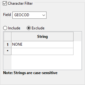
Select the Character Filter checkbox to limit the data by a character string found in the selected database field.
-
Select the database field from the Field drop-down list. Only character fields will be listed.
-
Decide whether you want to include or exclude the text string.
Important: The text strings are case sensitive and must be entered exactly as they will be found in the database.
-
Enter the string without quotation marks in the space provided. You can have multiple strings.
Example: In the image above, our database is populated with four GEOCOD values: TQ1, TQ2, TQ3, and NONE. We have opted to include all values except those samples which have a value as NONE. Any sample that contains a GEOCOD value of NONE will be excluded from our sample population.
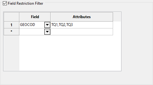
Select the Field Restriction Filter checkbox to restrict the data by field attribute.
-
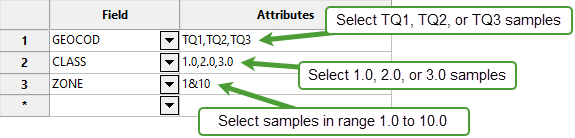
Select a Field from the drop-down list and enter applicable selection criteria to filter the samples by in the Attributes column.
Include spaces in the entries in the Attributes column only if spaces are included in the desired field values.
When entering a range, always enter the smallest number specified before the largest number.
Example:
-792&-720since-792is smaller than-720. This range is evaluated as-792.0 ≤ VALUE < -720.0.
Estimation Result Variables
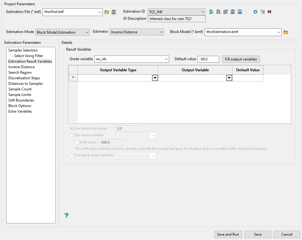
Use this panel to select the grade variable you want to run estimations on, along with any additional output variables. The only variable that is required is the initial grade variable. All of the output variables are optional and not needed to run your estimations.
Follow these steps:
-
First, select the primary variable you want to use for the estimations by selecting it from the Grade variable drop-down list.
Only valid variables will be displayed in the list.
-
Enter a default value for blocks that are not estimated.
-
Select any output variables you want to include in your estimation run. Depending on which estimation method you are using, the available output variables will change. The table below shows the entire list of output variables and the estimation methods in which they are used.
To quickly populate the table with all the variables, click the Fill output variables button.
Output Variable Type Output Variable Default Value ID SK OK IK UC Distance to Closest Sample (Anisotropic) au_ids_dist_c_an -99.0 * * * * Distance to Closest Sample (Cartesian) au_ids_dist_c_ca -99.0 * * * * Flag when Estimated au_ids_flag_variable 0.0 * * * * * Grade of the Closest Sample (Anisotropic) au_ids_grade_c_an -99.0 * * * * Grade of the Closest Sample (Cartesian) au_ids_grade_c_ca -99.0 * * * * Maximum Weight au_ids_max_weight -99.0 * * * Minimum Weight au_ids_minimum_weight -99.0 * * * Number of Holes au_ids_num_holes 0.0 * * * * * Number of Samples au_ids_num_samples 0.0 * * * * * Sample Coeff. of Variation au_ids_sample_coeff -99.0 * * * Sample Grade Minus Estimation au_ids_sample_grade_diff -99.0 * * * Sample Mean au_ids_sample_mean -99.0 * * * Sample Standard Deviation au_ids_sample_stddev -99.0 * * * Sample Variance au_ids_sample_variance -99.0 * * * The first column labelled Output Variable Type shows a description of the variable. This field cannot be edited.
The second column labelled Output Variable is the variable name that your block model will use. This field can be edited if desired.
Note: The name of a variable can have a maximum of 30 alphanumeric characters. The variable, which can only be entered using lowercase characters, must start with a letter and can only contain alphanumeric characters and/or underscores, for example,
variable_1.This is followed by the Default Value. This field can also be edited.
-
If you are using Simple Kriging as your estimation method, the option to manually define a mean will be enabled.
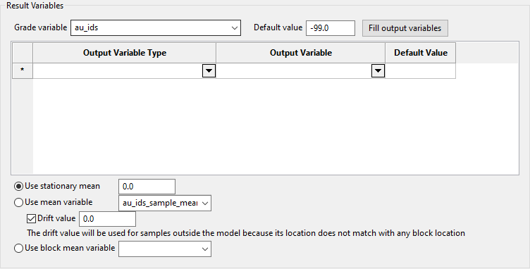
There three options to choose from.
-
Use stationary mean - Select this option if you want to manually define the stationary mean value.
-
Use mean variable - Select this option to take the locally varying mean into consideration. The mean variable is used for the sample mean and the block mean.
With this option, you can set the default value for all samples that are located outside the model area by entering a value into Drift value.
Note: The mean variable value is used if a block is found on XYZ coordinates (of the sample), and the stationary mean value is used if not. In earlier version of Vulcan these were exclusive. To keep the previous behaviour, set a value of 0.0 for the stationary mean.
-
Use block mean variable - Select this option to use the variable that holds just the block mean and not the sample mean.
-
Inverse Distance
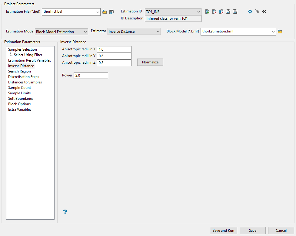
Use this panel to enter the anisotropic weightings applied to each direction of the search axes. The panel will display different options depending on whether you are using inverse distance or kriging methods for your estimation.
Follow these steps if you are using Inverse Distance.
-
In the space provided for Anisotropic Radii, enter the weightings for the X, Y, and Z directions. These weightings are a ratio of the lengths of the major, semi-major and minor radii. Thus the major (X) axis weighting is 1 (one), the semi-major (Y) axis weighting is the length of the major radius divided by the length of the semi-major radius, and the minor (Z) axis weighting is the length of the major axis radius divided by the length of the minor axis radius. Please note that it is possible to use equivalent ratios. That is 1:0.5:0.2 is the same as 10:5:2. The weightings are the inverse of the radii ratios.
Example: If the ratio is 1:0.5:0.2, then the weightings are 1, 2 and 5. The Distances to Samples panel (in Grade Estimation) and the New Estimation File option uses these weights for the Anisotropic distance derived from the anisotropic weights option.
If desired, you can click Normalise to calculate the anisotropic weightings normalised to the search radii. The distances used here are those entered into the Standard Major, Semi-major, and Minor axis settings found on the Search Region pane. You may still edit the weightings.
Example: If the ratio is 1:0.5:0.2, then the weightings are 1, 2 and 5. The Distances to Samples panel (in Grade Estimation) and the New Estimation File option uses these weights for the Anisotropic distance derived from the anisotropic weights option.
-
Enter the power to use on the inverse distance by entering the number in the Power textbox. A value of 2.0 means inverse distance squared while a value of 3.0 means inverse distance cubed, etc.
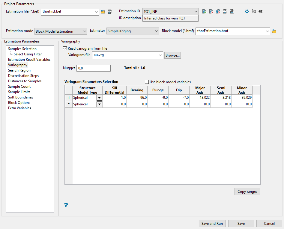
Variography
-
Select a variogram file. This step is optional. You can choose to enter the variogram information directly into the table if you desire to do so. To select the file, use the drop-down list labelled Read variogram from file, or click the Browse button if the file is located somewhere other than your current working directory.
All the files that have a (.vrg) extension will be shown in the list.
Note: To generate a variogram file, you can use an exported file from the Data Analysis tools located in the Analyse menu.
-
Enter the Nugget. This represents the random variability and is the value of the variogram at distance (h) ~ 0.
-
Complete the table defining the variogram parameters to be used. Enter the information by typing into the space provided for each column.
Tip: If you want to use block model variables instead, enable the Use block model variables checkbox, then use the drop-down lists to populate each field. The drop-down lists will automatically display all eligible variables from the block model selected at the top of the panel.
Explanation of table columns
Structure model type
Spherical
This type is the most commonly used for ore deposits. They exhibit linear behaviour at and near the origin then rise rapidly and gradually curve off.
Exponential
This type is associated with an infinite range of influence.
The sill is reached at the specified range parameter. In release 3.2 and earlier, users were required to enter a range parameter of one-third the practical sill range. To use this model, enter the practical distance of the sill as a range parameter. For backward compatibility, see the Exponential Model 3.
Gaussian
This type exhibits parabolic behaviour at the origin and, like the spherical model, rises rapidly. The Gaussian type reaches its sill smoothly, which is different from the spherical model, which reaches the sill with a definite break. The Gaussian model is rarely used in mineral deposits of any kind. It is used most often for values that exhibit high continuity.
In release 3.2 and earlier, users were required to enter a sill range of 3 times the actual sill range. To use this model, enter the effective range of the sill. For backward compatibility, see the Gaussian model 3.
Linear
This type is a straight line with a slope angle defining the degree of continuity.
De-Wijsian
This type is a representation of a linear semi-variogram versus its logarithmic distance.
Power
This type is computed as M - d**p where M = the maximum correlation defined as 1000.0, d = distance from the origin, p = model power. For this model type only the power p is the major axis radius. Adjust the size of the ellipsoid so that the major axis is the desired power. The size of the ellipsoid for this model does not change the calculation of the variogram.
Exponential Model 3
This is an un-normalised exponential model for compatibility with release 3.2 and earlier. This variogram will have the practical sill at three times the distance entered as range parameter.
Periodic
This is a sine wave with one complete period over the effective range. This model is not commonly used because it can cause samples at greater distances to have higher correlation.
Gaussian Model 3
This is an un-normalised Gaussian model for compatibility with release 3.2 and earlier. The input radius must be the effective radius multiplied by 3.
Dampened Hole Effect
Dampening is achieved by multiplying the covariance function by an exponential covariance, that acts as a dampening function.
Sill Differential
This represents the difference between the value of the variogram where it levels off and the nugget.
If you have a total sill of 1.0, and a nugget of 0.15, you want your sill differential to be 0.85 = (1.0 - 0.15).
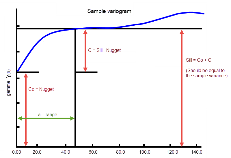
In the diagram, C0is the nugget, and C is the sill differential.
Bearing/Plunge/Dip
This is the bearing (Rotation about the Z axis), plunge (rotation about the Y axis) and dip (rotation about the X axis) of the variogram.
Major/Semi-Major/Minor Axis radii
This is the radii of the major, semi-major and minor axes of the variogram.
Search Region
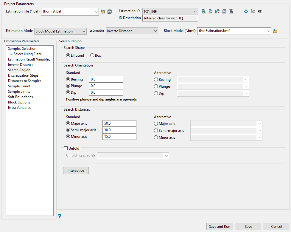
Use this panel to set the search direction and how far to look for samples.
Follow these steps:
-
Select the shape of your search area. Select Ellipsoid or Box.
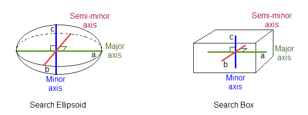
The major radius is "a", the semi-major radius is "b" and the minor radius is "c".
Note: The volume of a box with sides 2a, 2b, and 2c is about twice the volume of an ellipsoid with radii a, b, and c. Therefore, when using the box search you collect about twice as many sample points. This causes an estimation using a box search to take from two to eight times as much time as an estimation with a search ellipsoid.
-
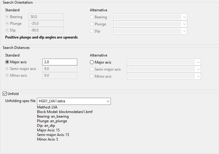
Set the search orientation.
The Bearing, Plunge, and Dip values are angles, in degrees, that specify the orientation of the search ellipsoid and orientation of variogram structures.
Care must be taken with these parameters as there are several common misunderstandings about their meaning.
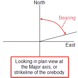
Bearing
Bearing is the angle of the Major axis as it rotates clockwise from the north. It is the angle of the strikeline of the orebody.
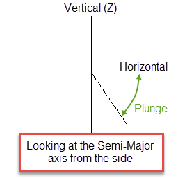
Plunge
Plunge is the angle of the Semi-major axis as it rotates around the minor axis. Note that the plunge should be negative for a downward pointing ore body.
Dip
Dip is the angle of the minor axis of an orebody as it rotates around the Major axis. Think if it as the angle that an orebody tips from side to side when looking down the strikeline.
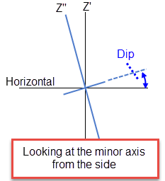
Note: The terms bearing, plunge and dip have been used by various authors with various meanings. In this panel, as well as kriging and variography, they do not refer to true geological bearing, plunge, and dip. The terms X', Y', and Z' axis are used to denote the rotated axes as opposed to X, Y, and Z which denote the axes in their default orientation.
-
Enter the dimensions of the search box. The search box has sides with length twice the numbers given. The major axis radius is the search distance along the axis of the ore body. The semi-major radius is the search distance in the ore body plane perpendicular to the ore body axis. The minor axis radius is the search distance perpendicular to the ore body plane.
NoteThe search radii are true radii. If you set your major search radius to '100', then the ellipsoid has a total length of 200. The following diagram shows the relationship between the axes with the ellipse in the default orientation (bearing 90°, plunge and dip 0.00°).
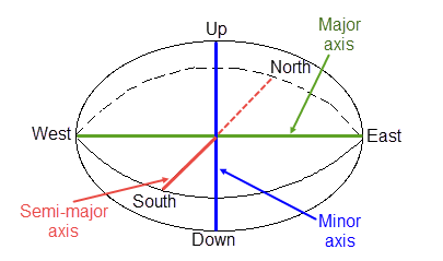
Relationship between radii
-
If you are using a tetrahedral model, you can select the Unfold checkbox to select a (*.tetra) file from the Unfolding spec file drop-down list. This list will contain all (*.tetra) files found within your current working directory. Refer to the Unfolding section for more information on tetrahedral modelling.
NoteWhen using an Unfolding spec file, the panel will read the type of method used in the Unfolding Model (LVA, Bend or Projection) and lock the panel options according to the parameters set in each of these methods.
-
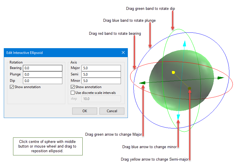
Click the Interactive button to display the Edit Interactive Ellipsoid panel define search ellipsoids on screen in Vulcan. Once defined in Vulcan, the parameters will then be written back into the panel.
Discretisation Steps

Use this panel to set the parameters for the discretisation steps that will be used.
Note: If you want data located at the block centroids to be used for block estimates, then run another estimation using a maximum of one (1) sample and storing the average distance to samples. Then run a block calculation or a script on the block model and assign the new grade value to your results with the condition that the average distance is zero (0) (provided the default is not set to 0).
Estimates are always made as block estimates. This means that if you have data at exactly the block centre, that data is not used as the value for the block in ordinary kriging or inverse distance. However, as the value of the data at a block centroid for the inverse distance method attains nearly all of the weighting, the estimate closely approximates the data value. Instead, all samples are used for kriging and inverse distance and an estimate is produced in the usual manner.
Note: The panel is displayed if you have selected Inverse Distance, Simple Kriging, or Ordinary Kriging as an estimation method. It is not available if you are using Uniform Conditioning.
Follow these steps:
-
Enter the number of steps you want to utilise into the spaces provided for Discretisation steps in X/Y/Z. The step sizes indicate how many grid points will be used inside a block or sub-block. Envisage uses the grid points for calculating block averages. For point kriging, each discretisation size should be set to 0 (zero). A large number of grid points can cause Envisage to run slowly. A 4 × 4 × 4 grid is usually sufficient. In no case should there be more than 10 000 grid points.
-
If you are using Inverse Distance as the estimation method, you can elect to use the average of discretised block distances to samples when using discretisation for ID weight calculation, by enabling the Average distance for discretised blocks option.
Note: This option is not available if you are using kriging methods.
-
Decide whether you want to estimate sub-blocks as if they were the parent blocks. This means that instead of using the block extent of the sub-block, the estimation procedure uses the extent of the parent block. To do this, enable the checkbox Assign parent block values to sub blocks.
Suppose we have a primary scheme of block size of (50, 50, 50) and we are estimating a block whose extent ranges from (60, 30, 50) to (70, 40, 70). This block has sides of length 10, 10, and 20. The parent block that contains the sub-block ranges from (50, 0, 50) to (100, 50, 100). The parent block has sides of 50, 50 and 50 and has centre at (75, 25, 75). This block is estimated as if its centre were at (75,25,75) and as if its sides were 50, 50 and 50.
If you decide to use this feature, you are presented with three options:
Use model schema for parent size
Select this option to use the parent size blocks as they are defined in the block definition file.
Choose parent block size
Select this checkbox to enter the parent block size and specify the lengths of the block.
Note: If any type of block selection is used, then not all sub-blocks in a parent block have the same value. A sub-block is only estimated if it is selected by the block selection procedure.
Example: Suppose you have two zones,
OREandROCK.When you estimate blocks in theOREzone, only blocks actually in the ore zone are updated. Blocks in theROCKzone are not updated, even if they are in the same parent block.If you want all blocks in a parent block to have the same grade value, then you need to run grade estimation on all the sub-blocks. The easiest way to do this is to run grade estimation without any block selection conditions.
If the Choose parent block size checkbox is not selected, then the true block extents and sizes will be used instead.
Read parent block size from model
Select this option to define the parent block sizes using predefined variables in the block model. This option is useful if you have two or more zones (as in the example noted above in the description for Choose parent block size).
Distance to Samples
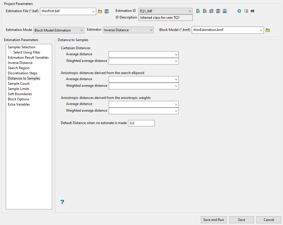
Use this panel to set the parameters to store the search distances used to look for your samples. Any, all, or none of the different distance measures can be stored by putting a block model variable name in the appropriate panel item. If you do not want to store a value, then leave the panel item blank.
Follow these steps:
-
Enter a variable name into the appropriate box. There are three different kinds of distances that can be stored:
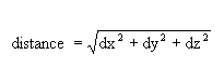
Standard Cartesian
The distance from the block centre is computed using the Pythagorean formula:
If no weighting is used, then each sample is given an equal weight. If weighting is used, then the weights used in grade estimation are applied. When performing indicator kriging, the weights of the first cutoff are used.
Anisotropic distance derived from the search ellipsoid
If your search ellipsoid is spherical (major, semi-major and minor radii are the same) this anisotropic distance is the same as the Cartesian distance. Suppose, however, that your search ellipsoid has radii of 100, 50 and 10. This means that points in the direction of the semi-major axis have their distances expanded by a factor of 2 = (100/50) and points in the minor direction have their distances expanded by a factor of 10 = (100/10). In general, anisotropic distances are computed as:
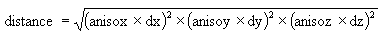
where
dx, dy, and dz are the distances in the major
semi-major and minor directions
anisox, anisoy, and anisoz are the anisotropic weighting factors
The anisotropic weighting factors cause any samples that lie on the surface of the search ellipsoid to have the same anisotropic distance, namely, the major axis radius.
Anisotropic distance which is derived from anisotropic weights
This option is only available when using the inverse distance method. When you define the inverse distance method you define radii that control the inverse distance weighting. If you normalise your inverse distance weights to the search ellipsoid radii, these distances are the same as the distances derived from the search ellipsoid.
Either unweighted or weighted distances can be stored. If unweighted, then all samples are given the same weight. If weighted, the weights used for grade estimation are applied.
Example: Suppose we are estimating a block and have two samples. Sample 1 is at a distance of 10 and Sample 2 is at a distance of 100. Suppose, also that Sample 1 has a weight of 0.95, and Sample 2 has a weight of 0.05. The unweighted distance is
(10+100)÷2or55. The weighted distance is(0.95×10 + 0.05×100)or14.5.In addition there are weighted and unweighted interpretations of each of these, for a total of six different kinds of distance.
-
Next, if you want to use a default that will be stored as an average distance if there aren't enough samples available to make an estimate, entering a number into Default distance when no estimate is made.
Sample Count
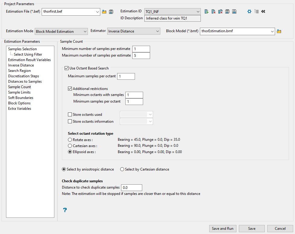
Use this panel to set the minimum and maximum number of samples that will be used to estimate the grade of a block.
Follow these steps:
-
Enter the lowest number of samples in the box labelled Minimum number of samples per estimate.
This is the minimum number of samples that needs to be found to generate an estimate. Blocks with less than this number of samples within the search ellipsoid or search box are assigned the default grade value.
-
Enter the largest number of samples in the box labelled Maximum number of samples per estimate.
This is the maximum number of samples to be used in any grade estimation. Up to 999 samples per estimate are allowed.
Example: The estimation program may find 30 samples near a block centre. If you had specified a maximum of 10 samples, then only the 10 samples closest to the block centre are used. The distance to the block centre is calculated by an anisotropic distance based on the search radii.
-
Decide whether or not to use an octant search. The space around a block centre is divided into eight octants by three orthogonal planes.
Note: An octant search is a declustering tool used to reduce imbalance problems associated with samples lying in different directions. If there are more samples in one direction than another, then this option limits the bias.
If want to use an octant search, enable the checkbox labelled Use Octant Based Search. This places a limit on the number of samples that can come from a given octant.
-
Enter the maximum number of samples from each octant to be used in the estimation in the box labelled Maximum samples per octant. Samples closest to the block centre are used first.
Note: The maximum number of samples per estimate always applies, regardless of the maximum samples per octant value.
-
Enable the checkbox labelled Additional restrictions if you want to limit the number of samples for octants. Then enter the number of minimum and minimum samples per octant.
The minimum octants with samples enables you to specify the number of octants that must contain samples for an estimate to be generated. The minimum samples per octant enables you to specify the number of samples per octant that needs to be found to generate an estimate. These two restrictions work together. An octant is considered filled if it contains at least the minimum number of samples per octant. The minimum number of octants with samples requires that at least that number of octants be filled.
If you set the minimum number of samples per octant to 2, the minimum number of octants to 3 and have the following number of samples per octant, there are two filled octants. As this is less than the minimum number of octants with samples, the default value is assigned to this block.
Octant Number
Number of samples per octant
Filled / Not Filled
0 1 Not filled 1 3 Filled 2 2 Filled 3 1 Not filled 4 1 Not filled 5 1 Not filled 6 1 Not filled 7 0 Not filled -
Enable the checkbox labelled Store octants used if you want to save the number of octants in a block model variable.
-
Enable the checkbox labelled Store octants information if you want to save information concerning which octants were used by each estimated block in a block model variable.
-
Select octant rotation type.
Rotate axes This consists of three planes perpendicular to axes that have been rotated 45° about the Z axis and 35° about the X' (X axis after rotation about the Z axis), this produces a set of planes in which the first has a bearing of 135°, the second has a bearing of 45° and is at angle of -55° to the horizontal and the third also has a bearing of 45°, but is at an angle of 35° to the horizontal. (See the diagram below.) Cartesian axes This consists of three planes perpendicular to the conventional Cartesian axes X, Y, and Z (or East, North, and elevation) axes. Ellipsoid axes This consists of three planes that are perpendicular to the major, semi-major, and minor axes of the search ellipsoid. 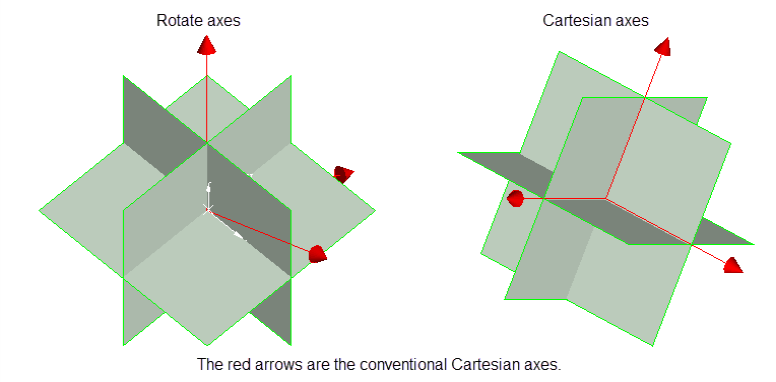
-
Select the method by which the samples will be measured by choosing either Select by anisotropic distance or Select by Cartesian distance. The samples are sorted by distance (either anisotropic or Cartesian) prior to the samples being limited. This ensures that the closest samples are kept.
-
To prevent the same sample from being used more than once, enter the distance to use in Distance to check duplicate samples. Samples less than or equal to the specified distance value are considered to be duplicates, resulting in the entire grade estimation process being stopped. You can disable this feature by specifying a distance value of
'-1'.
Cutoff
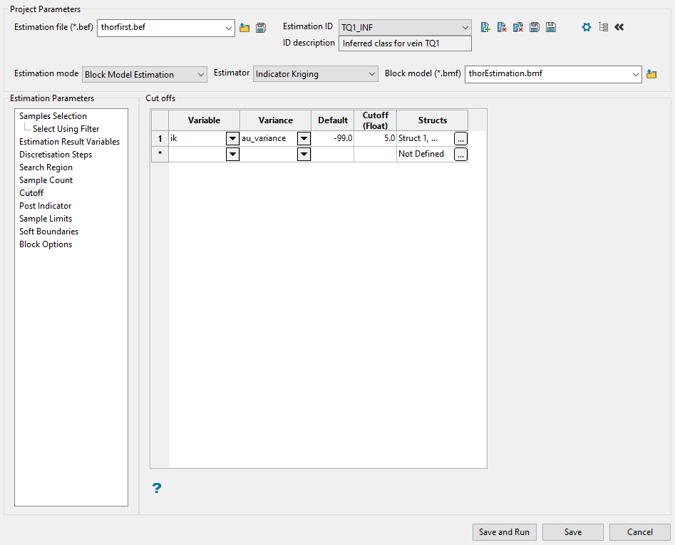
Use this panel to set the parameters for the cutoff you want to evaluate.
-
Enter the block model variable in which to store the indicator variable by selecting it from the Variable drop-down list.
-
Specify the kriging variance from the variogram model for this cutoff by selecting it from the Variance drop-down list.
-
Enter the Default value (the default value is '0'). This value is used for the indicator and variance when the block is not estimated.
-
Enter the grade Cutoff level. The cutoffs should be entered from lowest cutoff to highest cutoff. A sample value equal to the cutoff is considered to be in the interval above the cutoff.
-
Set up the structures by clicking the icon in the Structs column.
Start by selecting a variogram file. This step is optional. You can choose to enter the variogram information directly into the table if you desire to do so. To select the file, use the drop-down list labelled Read variogram from file, or click the Browse button if the file is located somewhere other than your current working directory.
All the files that have a (.vrg) extension will be shown in the list.
Note: To generate a variogram file, you can use an exported file from the Data Analysis tools located in the Analyse menu.
Next, enter the Nugget. This represents the random variability and is the value of the variogram at distance (h) ~ 0.
The next step is to complete the table defining the variogram parameters to be used. Enter the information by typing into the space provided for each column.
Tip: If you want to use block model variables instead, enable the Use block model variables checkbox, then use the drop-down lists to populate each field. The drop-down lists will automatically display all eligible variables from the block model selected at the top of the panel.
Explanation of table columns
Structure model type
Spherical
This type is the most commonly used for ore deposits. They exhibit linear behaviour at and near the origin then rise rapidly and gradually curve off.
Exponential
This type is associated with an infinite range of influence.
The sill is reached at the specified range parameter. In release 3.2 and earlier, users were required to enter a range parameter of one-third the practical sill range. To use this model, enter the practical distance of the sill as a range parameter. For backward compatibility, see the Exponential Model 3.
Gaussian
This type exhibits parabolic behaviour at the origin and, like the spherical model, rises rapidly. The Gaussian type reaches its sill smoothly, which is different from the spherical model, which reaches the sill with a definite break. The Gaussian model is rarely used in mineral deposits of any kind. It is used most often for values that exhibit high continuity.
In release 3.2 and earlier, users were required to enter a sill range of 3 times the actual sill range. To use this model, enter the effective range of the sill. For backward compatibility, see the Gaussian model 3.
Linear
This type is a straight line with a slope angle defining the degree of continuity.
De-Wijsian
This type is a representation of a linear semi-variogram versus its logarithmic distance.
Power
This type is computed as M - d**p where M = the maximum correlation defined as 1000.0, d = distance from the origin, p = model power. For this model type only the power p is the major axis radius. Adjust the size of the ellipsoid so that the major axis is the desired power. The size of the ellipsoid for this model does not change the calculation of the variogram.
Exponential Model 3
This is an un-normalised exponential model for compatibility with release 3.2 and earlier. This variogram will have the practical sill at three times the distance entered as range parameter.
Periodic
This is a sine wave with one complete period over the effective range. This model is not commonly used because it can cause samples at greater distances to have higher correlation.
Gaussian Model 3
This is an un-normalised Gaussian model for compatibility with release 3.2 and earlier. The input radius must be the effective radius multiplied by 3.
Dampened Hole Effect
Dampening is achieved by multiplying the covariance function by an exponential covariance, that acts as a dampening function.
Sill Differential
This represents the difference between the value of the variogram where it levels off and the nugget.
If you have a total sill of 1.0, and a nugget of 0.15, you want your sill differential to be 0.85 = (1.0 - 0.15).
In the diagram, C0is the nugget, and C is the sill differential.
Bearing/Plunge/Dip
This is the bearing (Rotation about the Z axis), plunge (rotation about the Y axis) and dip (rotation about the X axis) of the variogram.
Major/Semi-Major/Minor Axis radii
This is the radii of the major, semi-major and minor axes of the variogram.
Post Indicator
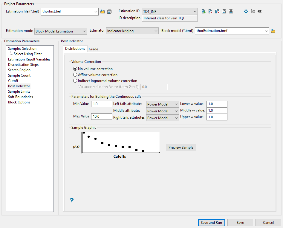
Use this panel to set up the distribution. After calculating the indicator values for the cutoffs, you will have a discrete distribution. You can extend the discrete distribution to a continuous distribution with a certain mean and variance. Because of the difference between point and block samples, the variance of the distribution is too large. To compensate for this, it is desirable to reduce the variance of the distribution.
-
Choose the type of variance reduction you want to apply by selecting one of the three Volume Correction methods: No volume correction, Affine volume correction, Indirect lognormal volume correction.
The distribution is linearly rescaled by the square root of the variance reduction factor while maintaining the same mean value.
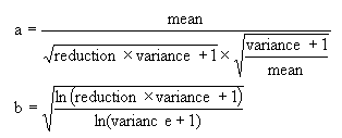
This adjusts the distribution, preserving the mean and changing the variance, assuming that the distribution is lognormally distributed. The cutoffs of the distribution are replaced by cutoffs at

where:
cut is a cutoff level
and a and b are parameters that Vulcan calculates to change the variance.
The cutoffs are further adjusted to restore the mean of the distribution.
Note: The adjustment of the cutoffs does not change the cutoffs used for computing the indicators, only the cutoffs used for computing the distribution statistics.
The parameters a and b are calculated as:
-
If you select Indirect lognormal volume correction, you will need to also enter a Variance reduction factor within the range of 0 to 1. The variance of the distribution is multiplied by this factor.
The Post Indicator process can construct a continuous distribution from the discrete distribution produced by indicator kriging. To do this, several assumptions are made that are controlled by the following parameters.
-
Enter the minimum and maximum thresholds by the lowest and highest grade value in the spaces labelled Min value and Max value.
For the minimum of the distribution, enter the lowest grade value in the distribution. This should be less than the lowest cutoff. Often zero (0) or the minimum detectable limit are appropriate minimum values.
For the maximum of the distribution, enter the highest grade value in the distribution. This should be greater than the highest cutoff. Increasing this value causes higher values to be produced when selecting grade values from above the highest cutoff.
-
Enter the left tail distribution parameter. This controls the shape of the curve from the minimum of the distribution to the lowest cutoff. If the parameter is '1', then the curve is a straight line between the minimum distribution value and the lowest cutoff. If it is less than 1, then the distribution is skewed to the left (the curve is above a straight line). If it is greater than 1, then the distribution is skewed to the right (the curve is below a straight line).
The choices are:
-
Linear Model
-
Power Model
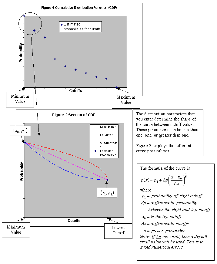
Enter the middle interval distribution parameter. This is like the left tail distribution parameter, but applies to the intervals between the lowest cutoff and the highest cutoff.
Enter the right tail distribution parameter. This is like the left tail distribution parameter, but applied to the intervals between the highest cutoff and the maximum of the distribution.
The choices are:
-
Linear Model
-
Power Model
-
Hyperbolic Model
-
-
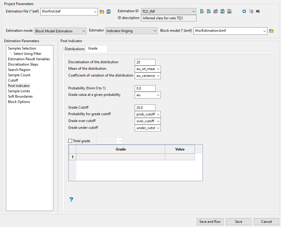
Enter the number of samples to be used when computing distribution means in the space labelled Discretisation of the distribution. A discretisation of 20 is usually fairly reasonable. Using a lot of discretisation can result in slower computing of distribution means without producing a more meaningful or more accurate number. If discretisation of 20 is used, then the distribution is sampled at steps of 5 percent from 2.5 percent to 97.5 percent.
Note: This would miss the upper tail in the 98 and 99'th percentiles.
Having defined the parameters above, the following results can be computed from the continuous distribution. The total grade result is not computed from the continuous distribution.
-
Select the variable for the computed mean of the continuous distribution from the drop-down list labelled Mean of the distribution.
-
From the drop-down list labelled Coefficient of variation of the distribution, select the variable for the computed coefficient of variation of the continuous distribution after variance reduction, if any, has been applied. The coefficient of variation is the standard deviation divided by the mean.
-
Select the variable for the grade in the distribution, after variance reduction. Enter a probability in the space labelled Probability (from 0 to 1), then select the variable for the grade from the drop-down list labelled Grade value at a given probability. For example, using a probability of 0.01 causes the top 1 percent grade value to be stored in this variable.
-
Enter a Grade Cutoff.
-
Select the variable in which to store the Probability for grade cutoff.
-
Select the variables in which to store the average grade in the distribution above and below the given grade cutoffs.
-
Select the variable in which to store the total grade for the distribution. The grade is computed using the parameters below. The total grade does not depend on the parameters used to extend the discrete distribution to a continuous one. The total grade is calculated by taking the difference in indicator variables that represents the probability of being in the given interval and multiplying by the assumed grade for the given interval. The sum of these interval grades is the total grade. The indicator values will have an order relations correction applied to them before the total grade is computed.
Sample Limits
Use this panel to limit the effect a high-valued sample will have on distant blocks.
Important: Using this option will not place a grade cap on the high-yield samples. It will prevent them from being used in the estimation completely.
The high-yield exclusion ellipsoid specified through this section of the Estimation Editor interface has its own major, semi-major, and minor axes that have the same orientation as the ellipsoid defined in the Search Region panel. When selecting the samples for the grade estimation, any samples within the high-yield exclusion ellipse can be chosen whether they are greater than or less than the threshold. However, between the smaller high-yield exclusion ellipse and the normal search region ellipse, only samples that are less than the threshold will be used.
Follow these steps:
-
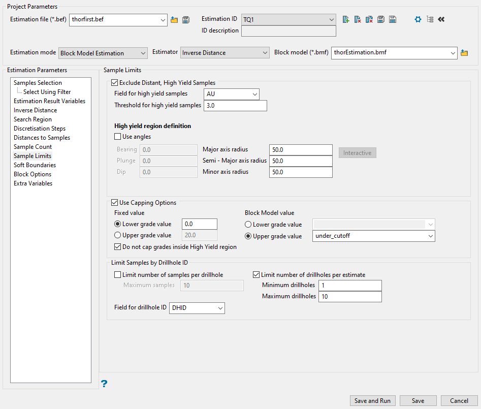
Enable the checkbox labelled Exclude distant, high yield samples to ignore sample values at or above the specified threshold and outside the specified ellipsoid.
-
Specify the database Field for high yield samples. It is usually the same as the input grade field. However, other fields can be used to achieve special sample limits.
-
Enter the threshold you want to use as a limit for high-yield samples. Only samples that are less than the threshold will be used.
-
Select Use angles if you want to use a customised orientation for the search ellipsoid. If you do not use this option, the samples will be selected using the ellipsoid defined in the Search Region panel.
Note: When a high yield region is defined, the value used puts a threshold on the samples outside of your specified distance and angle parameters. The high yield exclusion ellipsoid specified through this section of the Estimation Editor interface has its own major, semi-major and minor axes that have the same orientation as the ellipsoid defined through the Search Region section. When selecting the samples for the grade estimation, any samples within the high yield exclusion ellipse can be chosen whether they are greater than or less than the threshold. However, between the smaller high yield exclusion ellipse and the normal Search Region ellipse, only samples that are less than the threshold can be chosen. This is commonly used to avoid estimation from high gold nugget values to distant blocks.
Example: Using the settings in the screenshot above, we have several high-value samples that we would still like to use in our estimation and they outside of our high value spatial limits, so we set the Threshold value to 20. Then, we set our XYZ distance and rotation. Within that bubble, the high-value samples will be used without capping. Outside of that bubble, the value will be reduced to 20.
-
Enter the search distance into the spaces provided for Major, Semi-Major, and Minor axes radii.
Click the Interactive button to display an ellipsoid that can be edited by manipulating it with the mouse or entering the rotation and axis parameters directly.
-
Select Use Capping Options to set threshold values for the lower and upper grade values that will be used in your estimations.
You can use a Fixed value or use a Block Model value.
-
Select Do not cap grades inside High Yield region if you do not want a threshold applied to the region specified in Step 4 above.
-
If you want to limit how much influence a single drillhole or its samples will have, there are two methods you can apply: Limit number of samples per drillhole and Limit number of drillholes per estimate.
Note: When you select Limit number of drillholes per estimate, both the minimum and maximum number of drillholes per estimate must be specified. If you would like to apply only one of these parameters simply set the other parameter to an appropriate value. That is, if only the minimum parameter is required set the maximum to be greater than the maximum samples per estimate, or something like 99999. Similarly, if only the maximum parameter is required set the minimum to be 0 or 1.
-
Specify the name of the database field containing the drillhole name by selecting the field from the drop-down list labelled Field for drillhole ID. The default is DHID.
-
Enable the option Use Key Sample Limits to restrict samples based on the criteria you enter into the table. For example, you could use 10 samples for your estimation but limit the number of samples that come from RC drilling to just two samples.
-
Select the database field to evaluate.
-
Select the operator.
-
Enter a value.
-
Enter the number of samples allowed if the condition is TRUE.
-
Soft Boundaries
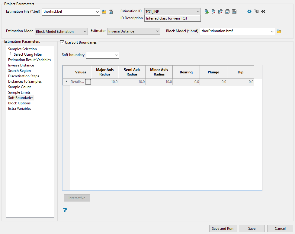
Use this panel to setup soft boundaries. Sometimes samples that are at a different estimation domain share similar grade properties when they are located close to the limit between the domains. This is often known as a soft boundary between the domains. In this case, it could be useful to include samples from a different domain but only at short distances from the blocks in the current domain.
Follow these steps:
-
Select this checkbox labelled Use soft boundaries to make the rest of the panel available.
-
Enter or select from the Soft boundary drop-down list the variable that will be used as a criteria to identify the estimation domains. The list is populated with the names of the database fields.
-
If you want block model variables to be used as radii for restricted search ellipsoid or the bearing, plunge, and dip values of the restricted search region, click the option labelled Use block model variables. All the block model variables will populate the drop-down list of the respective fields.
Explanation of table headings:
Values
Click on this field or select
 to display the Values panel.
Enter the values associated with the selected soft boundary. This panel will differ depending on whether the current boundary has a number or character value associated with it. Samples that have the values in this list for the soft boundary variable will be forced to use the ellipsoid specified in the next six boxes.
Major/Semi/Minor axis radius
Enter the radii for the restricted search ellipsoid or select a block model variable from the drop-down list.
Bearing/Plunge/Dip
Enter the bearing, plunge, and dip of the restricted search region or select a block model variable from the drop-down list.
Note: If the sample selection criteria does not allow for samples in soft boundaries domains to be selected, then no samples will be applied to the definitions specified here.
-
Click the Interactive button to display the Edit Interactive Ellipsoid panel define search ellipsoids on screen in Vulcan. Once defined in Vulcan, the parameters will then be written back into the panel.
Note: Clicking on a row to highlight it will enable the Interactive button.
Block Options
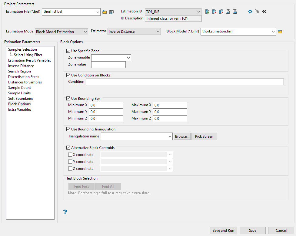
Use this panel to set up various block options.
Available options.
Select this checkbox to limit the estimation to those blocks where a specified variable equals a certain value. Both the variable and the value are forced to be lowercase.
Select this checkbox if you only want to apply a condition to the blocks to be estimated. A single condition can contain up to 132 alphanumeric characters. For a condition to contain more than 132 alphanumeric characters, you will need to manually edit the (.bef) file. Refer to Appendix B of the Vulcan Core documentation for a list of available operators/functions.
Select this checkbox to restrict the estimation to those blocks whose centroids lie within a specified range of co-ordinates. Enter the minimum and maximum co-ordinates (in the X,Y and Z directions). These co-ordinates are offsets from the origin of the block model (that is, block model co-ordinates).
Select this checkbox to limit the estimation to those blocks that lie within a specific solid triangulation. The triangulation name can either be manually entered or selected from the drop-down list. Click Browse to select a file from another location. You can also select loaded triangulations from the screen by clicking the Pick Screen option.
You have the ability to select block model variables for the blocks X, Y and Z centre coordinates. Each is optional, i.e. you can select one of the axis to be replaced only. In most cases, you will use Z to follow a sub-horizontal surface, but there may be cases on a different plane.
Note: During the grade estimation process, any blocks that have been selected but don't get an estimation value will receive the grade estimation default value. All blocks that have not been selected will retain their block creation default value. As a result, you could end up with two default values within the block model. If block selection criteria has not been specified, i.e. all blocks are selected, then the blocks not receiving an estimated value will have their block creation default value overwritten with the grade estimation default value, that is, one default value exists.
Localisation Strategy
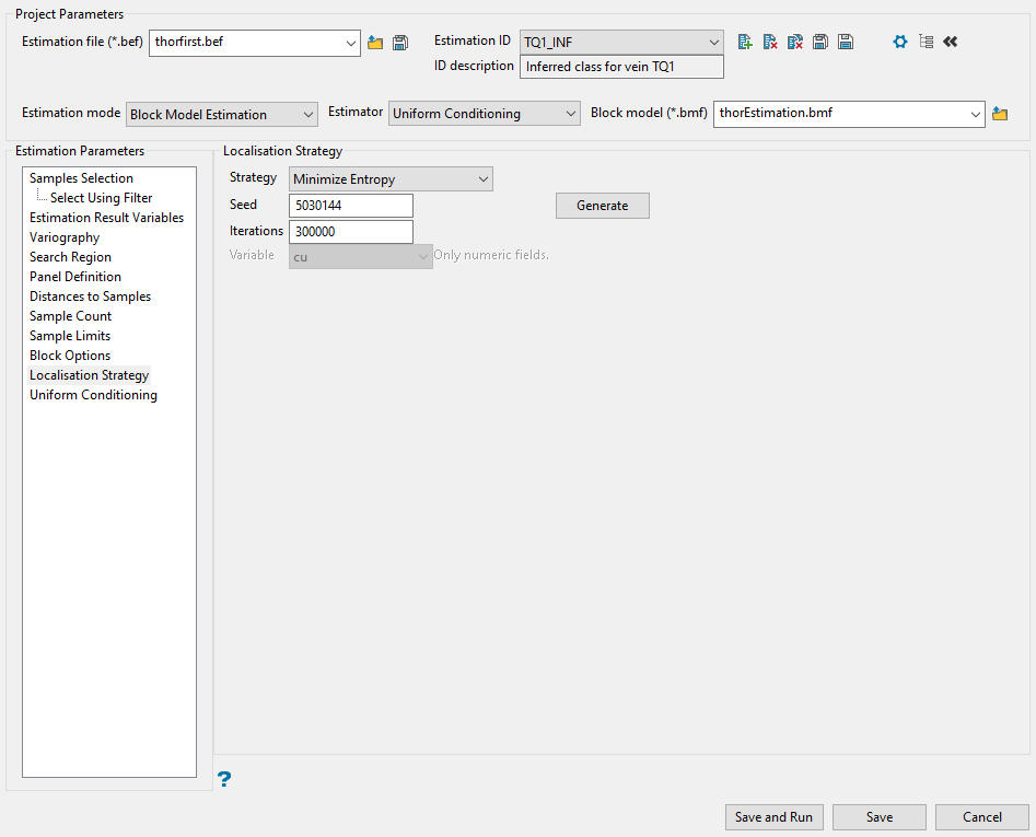
Use this panel to set the parameters for the estimation run. You will need to select the localisation strategy, seed, and number of iterations of the estimation.
-
Select the localisation strategy from the drop-down list labelled Strategy. There are four types to choose from:
Minimize Entropy
This method attempts to reduce randomness by comparing blocks within a panel. It will systematically swap the values of the blocks within a panel two at a time, and if the swap results in less randomness then it will keep the swap. The number of iterations is the number of swaps it will perform.
Randomly
Places the resulting values back into the model randomly.
Rank by SMU Estimate
Places the resulting values back into the model ranked according to the results of the existing SMU model. In other words, where the SMU model estimated the highest values the localisation strategy will place its highest values. Where the SMU model estimated its lowest values the localisation strategy will place its lowest values, and so on.
Secondary Data
Places the resulting values back into the model ranked according to a chosen secondary data source. It can be anything, such as LECO values, fuel values or rock type.
-
Enter a Seed. If you selected Minimize Entropy or Randomly as your strategy, you can enter your own number or click the Generate button to produce a random seed.
Note: A seed is not used with the Rank by SMU Estimate or Secondary Data strategies.
-
Enter the number of simulations in the space labelled Iterations.
Note: This is only used if you selected Minimize Entropy as your strategy.
-
If you selected Secondary Data as your strategy, you will need to select a variable from your block model from the drop-down list labelled Variable.
Uniform Conditioning
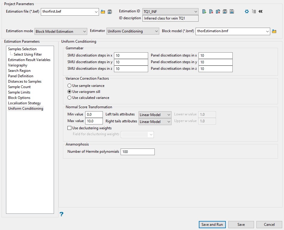
Gammabar refers to calculating the variance within the blocks.
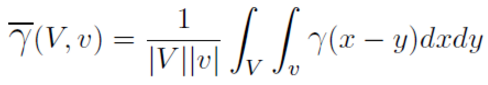
-
Enter the number of SMU discretisation steps for each direction. If the SMU represents a bench, then enter a 1 for the Z value.
NoteThe variance is obtained by discretising the block and calculating the average variogram value for all possible pairs. The X, Y, Z discretisation parameters control the number of pairs to consider. However, evaluating that integral directly is extraordinarily difficult, if not impossible. Therefore the variance within blocks is obtained by discretising the block with some number of sample points, and calculating the average covariance for all possible pairs within the block. The number of discretisation points can effect the final value slightly, but in practice 10 x 10 x 10 is generally accepted. (Too many discretisation points could lead to numerical precision issues; too few will give a poor estimate).
For uniform conditioning, we require the variance within both the SMU sized blocks and the panels. Therefore, you must specify the discretisation for both. In general the 10x10x10 does not need to be changed. One time you might change them is when doing 2d uniform conditioning (such as a single bench).
-
Enter the number of Panel discretisation steps for each direction.
Note: The panel are defined in the Panel Definition pane by one of three methods: manually defining the X,Y,Z inputs; Triangulated panel method; and Zone method. If you selected triangulated or zone methods then discretisation will not be available.
-
Select the Variance Correction Factors you wish to use. The variance correction factor (f) is the ratio of the block variance to the original sample variance.
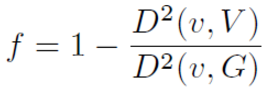
There are three options for sample variance:
-
Variogram sill - The default is to use the variogram sill, this is likely the correct choice. Recall that the dispersion variance (gammabar) is calculated with the variogram originally.
-
Sample variance - Use the (weighted) sample variance of the original samples.
-
Calculated variance - Use the variance calculated from fitting the sample anamorphosis (this is calculated from the hermite polynomials).
-
-
Set the parameters for the Normal Score Transformation.
-
Enter the minimum and maximum values in the spaces provided. These are the minimum and maximum values that a node can take when back transforming Gaussian values to grade units.
-
Select the type of model to use for the left and right tails.
The left tails attribute controls the shape between the lowest value in the transformation table and the minimum of the distribution. Linear and Power methods are displayed in the drop-down list.
The right tails attribute controls the shape between the highest value in the transformation table and the maximum of the distribution. Linear, Power and Hyperbolic methods are displayed in the drop-down list.
-
Enter the Lower w value and Upper w value in the space provided. A w value less than 1 leads to positive skewness, while a w value greater than 1 leads to negative skewness and a value equal to 1 is equivalent to a linear interpolation.
-
You also have the option of using a declustering weight. If you select this option, define the field used for the weights.
-
-
Set the Number of Hermite polynomials. By default this is set at 100, and should not be changed unless absolutely necessary.
Extra Variables
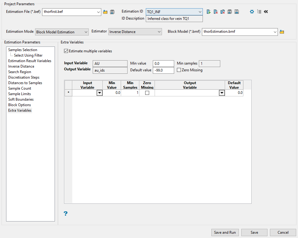
This panel allows you to apply the same weights to several sample variables.
Example: If you have several different metals that follow the same variography, then you may want to use the same weights for each of your metal variables.
Note: Your original sample variable and block model grade variable will always appear in this list.
Note: This panel is only available if you are using inverse distance, simple kriging, or ordinary kriging. It is not available if you are using indicator kriging or uniform conditioning.
Follow these steps:
-
Enable the checkbox labelled Estimate multiple variables.
-
Select the variable to which you want to apply the weighting from the Input Variable drop-down list.
-
By default, the values from Min Value, Min Samples, and Zero Missing are automatically copied over from the original variable. However, you can edit these by replacing the values in the cells.
-
Select the variable where you want to store the results by picking from the Output Variable drop-down list.
Explanation of table headings
Enter the sample variable from the mapfile or Isis composite database.
Enter the minimum value that is considered valid for this variable. Sample values below this value are considered missing. If your grade values are all positive and you use '-1' or '-9' as a missing data flag, putting 0 for this value is a good idea. The specified value can contain up to 3 decimal places.
When using inverse distance, it is acceptable to use the minimum value to eliminate samples with negative values. However, when kriging, this should not be done. Using restrictions under the Samples Database section is the correct way to exclude negative samples in the estimation. Here is an example of why:
Let's say that your estimation would use 3 samples to estimate a given block. One of these samples has a value of -99. When you use the minimum in the Extra Variables panel, it will select all three samples for the estimation (including the -99), then it will see the minimum of 0 and discard the -99 sample. This now leaves only two samples that would be used to estimate the block. Because of where the minimum comes into the process, it will not discard the sample and then search for another.
This is why you want to use sample restrictions instead. If in the search there are 3 samples that would be selected, but one is -99, the sample restriction set up to select samples greater than or equal to 0 will discard the -99 sample and look for another that meets the criteria.
Restrictions are applied as part of the search, but the minimum value is applied after the search phase is complete and discards whatever does not meet the minimum criteria. This is dangerous in kriging because the kriging matrix has already been calculated with the negative samples if sample restrictions are not being used, which can lead to incorrect values in the estimation.
Enter the minimum number of valid samples that are allowed for an estimate. If at least this many valid samples values are available, an estimate of this variable is made. This minimum may be less than the minimum number of samples.
Example: Suppose you specified a minimum of 5 samples per estimate and a minimum number of valid samples for a variable as 2. Then suppose that a block had 5 samples selected. This means that up to 3 of the samples could be missing and an estimation of that variable is still made. However, if 4 of the 5 samples were missing, then the estimate would not be made and the default value would be stored for that variable.
Select this checkbox to replace missing samples with zero and to use all of the weights. If this checkbox is not ticked, then the weights of the missing samples will be ignored and the remaining weights are re-normalised to sum to 1.
Note: This option does not apply to simple kriging.
Specify the variable in the block model to receive the weighted estimate. You must select one block model variable for every input variable you select.
Enter the default value. This value, which can contain up to 3 decimal places, is stored in the variable if it is less than the minimum number of valid samples available.

