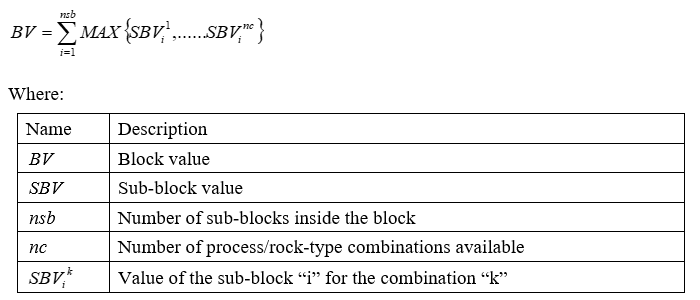
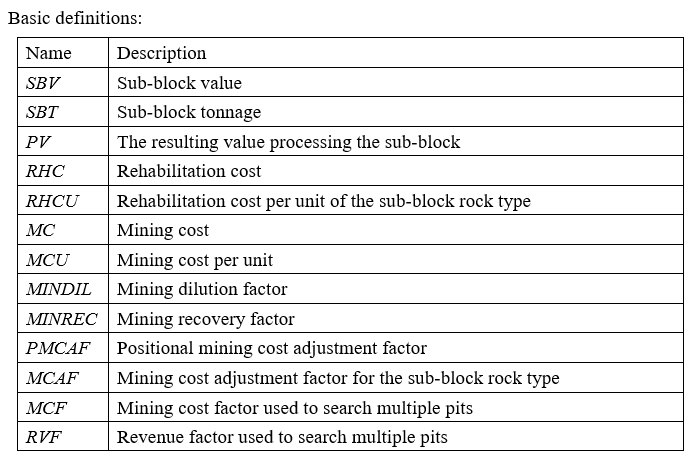
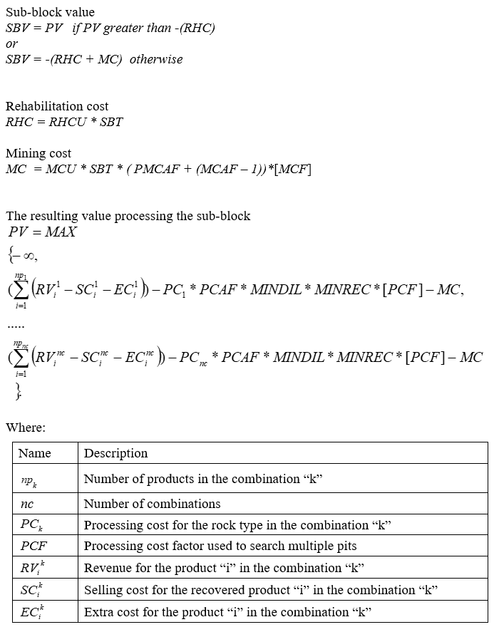
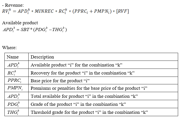
Edit
Use this option to develop the optimal pit limits of an ore body based on parameters defined in the interface. The pit optimisation process calculates the blocks that should be mined based on the criteria of maximising total economic value.
Important: Prior to using the Pit Optimiser option, a block model must exist with at least one grade variable to define the desired product(s). Additionally, load any subregions to the Vulcan workspace and prepare and load block model variables that you want to work with in the optimiser before launching the option.
Instructions
On the Block menu, point to Pit Optimiser, then click Edit....
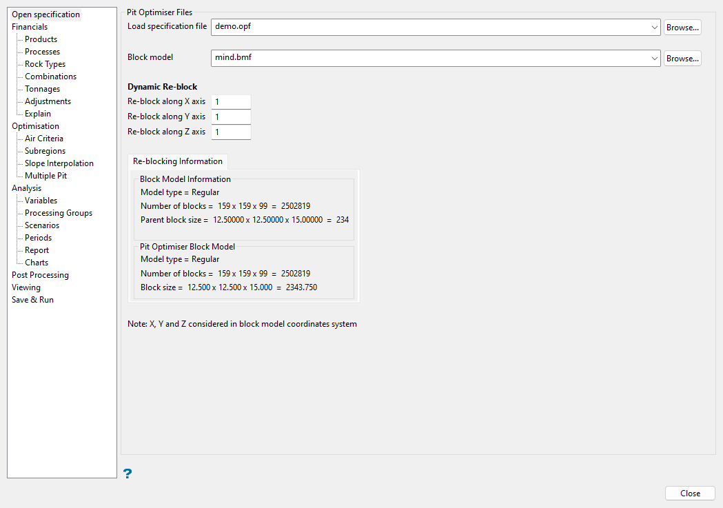
The Pit Optimiser interface is divided into the following key sections:
- Financials: Use this section to define parameters that will be used to obtain an economic value of each block. Product prices, process recoveries, rock types, process combinations, and costs are defined in this part of the interface.
- Optimisation: Use this section to set constraints for determining the optimal pit limits. Slope angles, subregions, air settings, and multiple pit settings are defined in this part of the interface.
- Analysis: Use this section to produce reports and charts based on the pits generated in the optimisation process.
- Post Processing: Use this section to export the economic value computed by the optimiser to block model variable. If multiple pits are generated, each pit uses a different economic value for each block. To account for this, this pane can be used to create a block model variable for each pit.
- Viewing: Use this section to generate triangulation shells and an animation file to visualise the pit, period, or phase output from optimiser.
- Save & Run: Use this section to save the parameters to a new or existing specification file (.opf), as well as perform the optimisation, analysis, and/or post processing.
Open specification
Use this initial pane to load an existing specification file, if applicable, and specify the block model name and dynamic re-blocking definitions.
Tip: Navigate to the Save & Run pane at any time to save the current panel inputs to a specification file, or to run the optimisation, analysis, or post processing with the current panel inputs. Note that running the Pit Optimiser will also save the specification file, overwriting the existing file with the current panel inputs.
Follow these steps:
-
Select an existing specification file (
.opf) from the Load specification file drop-down list, which contains all.opffiles in your current working directory. Click Browse... to select a file from another location.Note: It is not mandatory to load a specification file in this pane to use the Pit Optimiser interface. The Save & Run pane can be used to create a new file after the parameters have been set.
-
Select the Block model from which the variables will be read and the results written to from the drop-down list, which contains all
.bmffiles in your current working directory. Click Browse... to select a model from another location. -
Use the Dynamic Re-block section to make the optimiser and analysis group the existing blocks in the block model into larger re-blocked blocks, providing faster run times. Enter the number of blocks (in each direction) to group together for re-blocking purposes in the Re-block along the X, Y, and Z axis fields. The X, Y, and Z directions are considered in the block model coordinate system.
Example: If the original block model contains 1,000,000 blocks, each having dimensions of 10 x 10 x 10, then by defining a re-blocking dimension of 2 x 2 x 1 (i.e. two blocks are joined in the X direction, two in the Y direction, and the Z direction remains unchanged), the optimiser will work with blocks dimensioned 20 x 20 x 10. The optimiser will read every block in the nominated block model but will combine the block values into the larger block size for optimisation, which will reduce the number of blocks to consider to 250,000.
The Re-blocking Information section summarises the original block model and the pit optimiser block sizes.
Note: The blocks in the original block model will remain unchanged regardless of the re-block settings used, and the results from the optimiser will be stored within each of the original blocks.
Financials
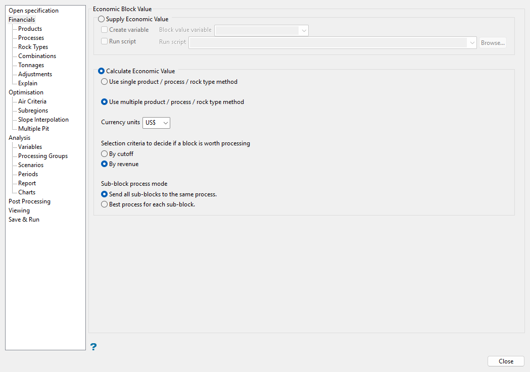
Use this pane to define the way the optimiser will treat each block in order to obtain the economic value.
Follow these steps:
-
Select either Supply economic value or Calculate economic value as the method to determine economic value of the blocks and set the applicable options.
-
Supply economic value: Select this option if the economic block value has been previously evaluated. The optimiser will use the economic value defined in the chosen block variable in the evaluation. A block that has a positive value is considered to be an ore block, a block with a negative value a waste block, and a block with an economic value of zero an air block.
Note: If this method is selected, the options to obtain multiple pits by product prices or economic factors are not available (i.e. the options in the Products, Processes, Rock Types, Combinations, and Tonnages panes in the Financials section, as well as the Use revenue/cost factors option in Multiple Pit pane in the Optimisation section will not be active).
-
Select an existing block model variable that represents the total value of the block from the Block value variable drop-down list. Alternatively, select the Create variable checkbox and enter a variable name to create a new block value variable from a script.
-
Select the Run script checkbox to use a block calculation file (
.bcf) to calculate the value of the selected Block value variable. If you select this option, select the script file from the drop-down list, or click Browse... to select a.bcffile from a location other than your current working directory.
-
-
Calculate economic value: Select this option to calculate the economic value of each block during the optimisation. By using this option, it is possible to change the economic scenario to obtain multiple pits for phase determination. Several parameters can be specified in order to adapt the block evaluation to the needs of different sites. Multiple pit/sensitivity analysis can be performed with all available options.
-
Select from the options below to use single or multiple product, process, and/or rock type methods in the optimisation:
-
Use single product/process/rock type method: Select this option if a single product variable and process method will be used in order to obtain the economic value of each block.
-
Use multiple product/process/rock type method: Select this option if multiple product variables, process methods, and/or rock types will be used to obtain the economic value of each block. This option allows the definition of different processes for different rock types with different recovery curves.
-
-
Set the Currency units by selecting from the available options in the drop-down list. This selection will be used for all costs in the parameters defined in the interface. Alternatively, a three-character, user-defined symbol can be manually entered.
-
Select the decision criteria to define if a block is minable (i.e. sent to the process plant) or not from the following options for Selection criteria to define if a block is worth processing:
-
By cutoff: Select this option to determine if blocks will be processed based on if they provide a value greater than zero. If the block provides a value that is negative when processed as ore, then the block is considered to be waste and is evaluated and treated as such.
Note: This option replaces the routing produced by the manual method. Although an actual cutoff is not computed or reported, the routing will be the same as if this method were used.
-
By revenue: Select this option to determine if blocks will be processed based on if they provide a value greater than the cost of the block when considered as a waste block. This option can be useful when defining pit phases or performing sensitivity analysis.
-
-
Select the Sub-block process mode from the following options to determine if a sub-block can be processed separately or not. The sub-blocks being considered can be either actual sub-blocks or blocks that were joined together by the dynamic re-blocking feature in the Open specification pane.
-
Send all sub-blocks to the same process: Select this option if the sub-block cannot be mined separately. This is useful for sub-blocked block models that were not dynamically re-blocked. The optimiser will send all sub-blocks to the process that gives the best value when all sub-blocks are sent to the same process.
-
Best process for each sub-block: Select this option to allow each sub-block to be treated as if it is mined separately and sent to a different process.
-
-
-
-
Advance to the applicable panes under the Financials group to define further parameters for the selected options.
Products
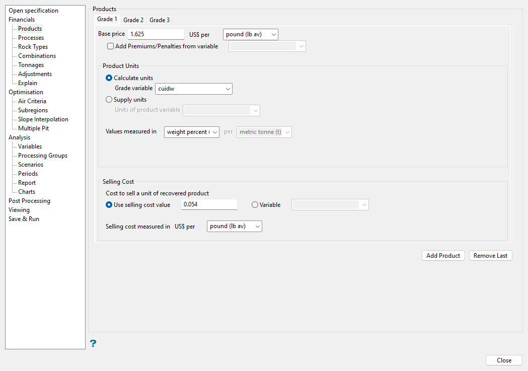
Use this pane to define the price and selling cost of the product(s), including the units.
Follow these steps:
-
Enter the Base price that defines the base case scenario used in order to obtain an income when selling the products units. This is also the base case to be used with decrements or factors in the Multiple Pit pane. The price is expressed in the currency selected in the Financials pane. Select the applicable base price mass units from the drop-down list.
Note: The base price mass units are the units used to report mass of the product in the analysis.
-
Select the Add Premiums/Penalties from variable checkbox to consider premiums/penalities calculated in a variable of the block model in the economic evaluation of the optimiser. Select the variable from the drop-down list. If this option is selected, it will be reflected in both the optimisation and analysis process. This variable should reflect the sum total of all premiums - all penalties for each block, in (currency units per product unit) and can be thought of as being directly added to the Base Price for each block.
Note: This option is useful for material like iron ore, where every block can have a premium or a penalty depending on the content of the elements inside each block (e.g. Fe, Si, etc.).
-
In the Product Units section, select whether to Calculate units or Supply units:
-
Calculate units: Select this option if the units of the product are not already stored in a block model variable and the units have to be calculated from a grade variable. Select from variables in the block model in the Grade variable drop-down list. This is the variable that contains the grade of the product in the block model.
-
Supply units: Select this option if the units of the product have been previously calculated in a block model variable. Select from variables in the block model in the Units of product variable drop-down list. This is the variable that contains the units of the product in the block model.
Note: If this option is selected, grades reported from the analysis will be in the units specified for Values measured in.
-
-
Select the Values measured in from the drop-down list as either the units of the grade or product units variable.
If the Calculate units option was selected previously, then you can specify two mass units to define the grade (e.g. grams per metric tonnes or carats per short ton). If one of the predefined grade units (i.e. weight percent or weight ppm) is selected as the first unit, then there is no need for a second mass unit and the second unit drop-down list will become unavailable.
If the Supply units option was selected previously with the product units specified, then only a single mass unit needs to be selected that corresponds to the units of the product in which the variable values are measured.
The following mass units may be used:
Unit symbol Description metric tonne (t) Metric tonnes kilogram (k) Kilogram gram (g) Gram carat (ct) Weight carat long ton (l ton) Long tonnes short ton (s ton) Short tonnes pound (lb av) Pound avoirdupois ounce (oz av) Ounce avoirdupois carat (ct av) Carat avoirdupois pound troy (lb tr) Troy pounds ounce troy (oz tr) Troy ounces carat troy (ct tr) Troy carats koku koku kann kann kinn kinn weight percent (%) Weight percentage weight ppm (ppm) Weight parts per million -
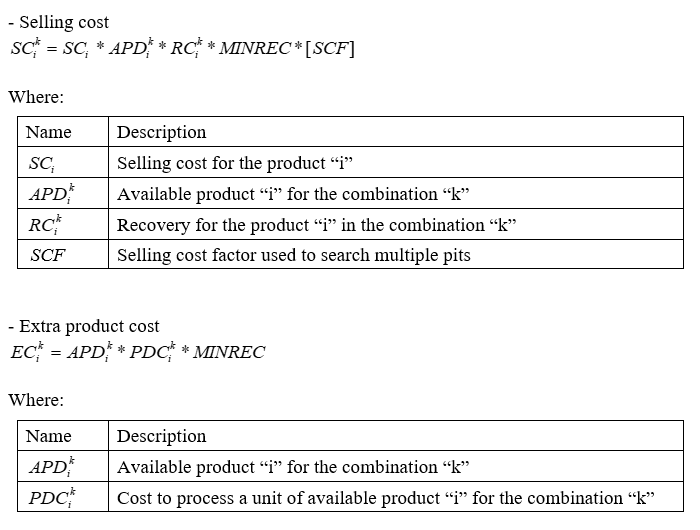
In the Selling Cost section, select from the following options to define the Cost to sell a unit of recovered product. This cost is applied after the recovery function has been applied to the block.
-
Use selling cost value: Select this option to enter a constant cost per unit of product.
-
Variable: Select this option if the selling cost varies for each block. Select the block model variable containing the cost per product unit from the drop-down list.
-
-
Specify the mass units in which the selling cost values are measured in the Selling cost measured in drop-down list.
-
If Use multiple product/process/rock type method is selected on the Financials pane, you have the option to click the Add Product button to create a new grade tab in the pane with an additional product. Complete the tab by repeating the steps above, choosing a different grade or product units variable to define. You can also click Remove Last to remove the last grade tab from the pane.
Note: After clicking either Add Product or Remove Last, the pane is restored to the first grade tab position. Select the desired grade tab to make edits.
Processes
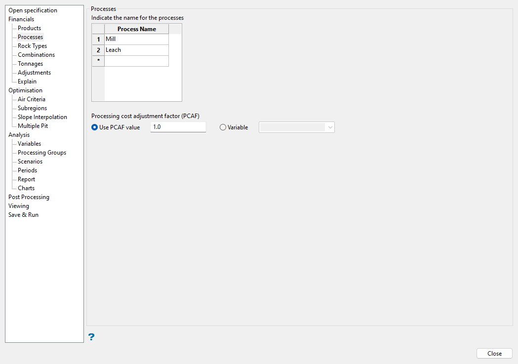
Use this pane to define processes that are used to extract the product as well as the adjustment factor for the processing cost.
Follow these steps:
-
If Use multiple product/process/rock type method is selected on the Financials pane, a grid will be available to enter a Process Name as an identifier for each processing method to be used in the optimisation. Up to five different process method identifiers can be used. These process names will be used later when defining parameters in the Combinations pane.
Note: This grid is only available if multiple processes are applicable, and the interface assumes a default process method when Use single product/process/rock type method is selected in the Financials pane.
-
Select from the following options for the Processing cost adjustment factor (PCAF):
-
Use PCAF value: Select this option to adjust the processing cost for each block by a constant factor specified in the associated field. This factor will multiply the processing cost for each block or sub-block for each process method. Enter a value of
1if no adjustment is needed. -
Variable: Select this option to choose a block model variable from the drop-down list that contains the factor to adjust the processing cost for each block. The value of this variable will be used to multiply the processing cost for each block or sub-block for each process method.
-
Rock Types
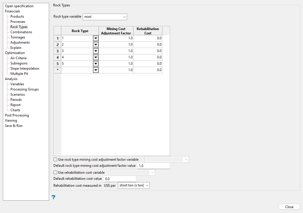
Use this pane to define rock type mining cost adjustment factors and rehabilitation costs. Rock types are not considered in a geological context here, but in a processing behaviour context. Rock types in the optimiser are used to define different behaviour for each process.
Follow these steps:
-
If Use multiple product/process/rock type method is selected on the Financials pane, select the Rock type variable in the block model from the drop-down list. This is the variable that contains the rock type values for each block or sub-block in the block model. Only integer or character variables are allowed.
Note: If Use single product/process/rock type method is selected on the Financials pane, the interface assumes a default rock type and the rock type variable and subsequent grid fields are not available.
For rock type values of interest, you can define specific parameters in the grid to be considered in the optimisation.
-
Specify values of interest in the Rock Type field. Enter a numeric rock type code if the variable is numeric or select values from the drop-down list if the variable is alphanumeric. Up to 10 rock type values can be specified in the grid.
Important: It is important to note that each Rock Type defined here will be selectable for the Combinations tab - not selecting a rock type here means it cannot be processed.
-
Enter the constant Mining Cost Adjustment Factor for each rock type. This factor will multiply the mining cost of the corresponding rock type.
-
Enter the Rehabilitation Cost that will be applied if a block is not processed (i.e. waste block) to remediate the unit of material after it has been mined.
-
-
Select the Use rock type mining cost adjustment factor variable checkbox if a different factor is defined for each block in the block model. Select the block model variable containing the rock type mining cost adjustment factor for each block from the drop-down list.
Note: If this option is selected, any defined constant mining cost adjustment factors are ignored.
Alternatively, if you do not select this checkbox and Use single product/process/rock type method is selected on the Financials pane, enter the value to be used as a single constant mining cost adjustment factor for each block in the block model in the Use mining cost adjustment factor value field. Enter a value of
1if the initial mining cost does not need to be changed. -
If Use multiple product/process/rock type method is selected on the Financials pane, enter the default mining cost adjustment factor in the Default rock type mining cost adjustment factor value field to use when a rock type code is found in the block model and has not been specified in the grid above, and when not using a mining cost adjustment factor variable. Enter a value of
1if the initial mining cost does not need to be changed. -
Select the Use rehabilitation cost variable checkbox if a different rehabilitation cost is defined for each block in the block model. Select the block model variable containing the rehabilitation cost for each block from the drop-down list.
Note: If this option is selected, any defined constant rehabilitation costs are ignored.
-
If Use multiple product/process/rock type method is selected on the Financials pane, enter the Default rehabilitation cost value to use when a rock type code is found in the block model and has not been specified in the grid above, and when not using a rehabilitation cost variable. Enter a value of
0if there is no need to consider the cost to rehabilitate.Alternatively, if you do not select this checkbox and Use single product/process/rock type method is selected on the Financials pane, enter the value to be used as a single constant rehabilitation cost for each block in the block model in the Use rehabilitation cost value field. Enter a value of
0if there is no need to consider the cost to rehabilitate.The rehabilitation cost will only be applied if a block is not processed (i.e. waste block) to remediate the unit of material after it has been mined.
-
Select the mass units in which the rehabilitation cost values are supplied from the Rehabilitation cost measured in drop-down list. This applies for both the constant or variable values.
See the Sub-block process mode under the Financials pane section of this page for more information on how parameters are incorporated into the mining cost.
Combinations
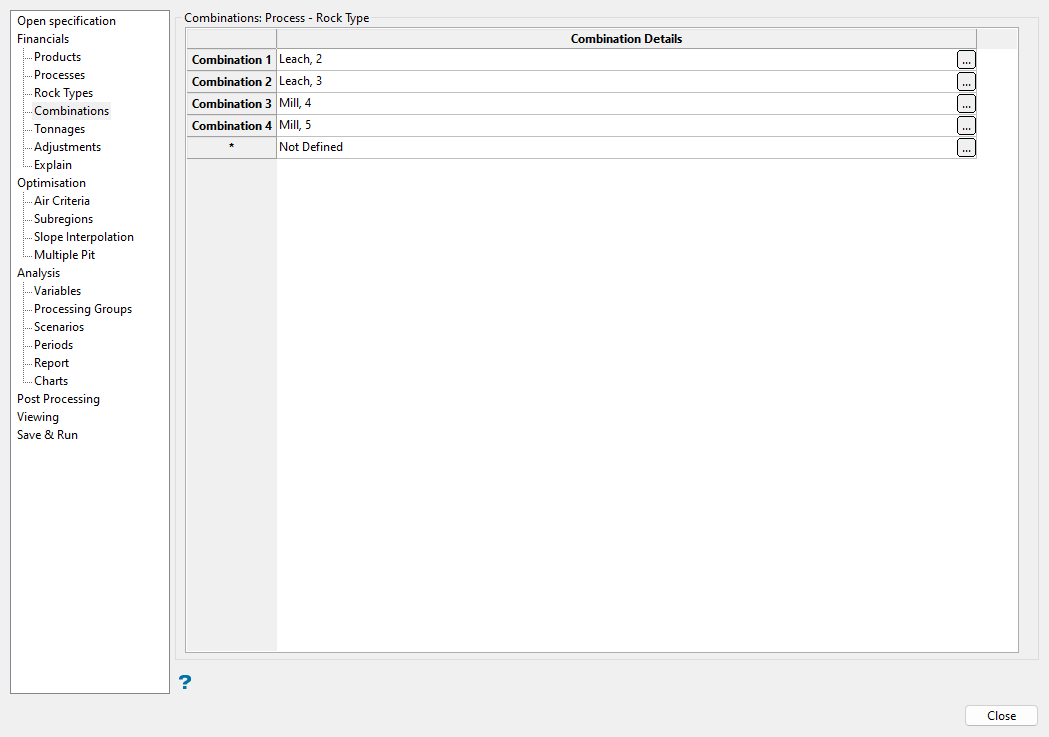
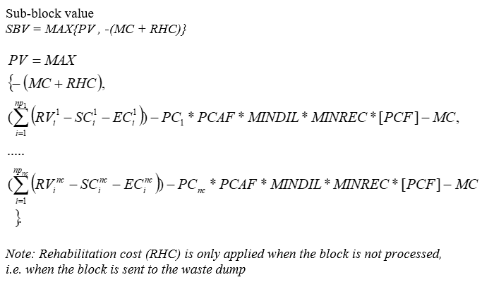
Use this pane to define process, rock type, and product combinations and their associated costs. You can also choose to consider contaminants, cut-off and threshold grades, process recovery, and cost to process available product in the combinations.
If Use multiple product/process/rock type method is selected on the Financials pane, it can be useful to define multiple combinations of products, processes, and rock types. The flexibility in the interface allows multiple products to be sent to the same process, and rock types can be treated differently. For instance, it is possible for a particular rock type to be suitable for different processes; however, the behaviour of the different elements in each process can differ. Recoveries could increase or decrease, treatment costs may vary, and products may be entirely ignored in some combinations of process and rock type. Rock types are not considered in a geological context here, but in a processing behaviour context.
For each block, only one Combination will be selected (highest profit). For example, a copper-gold deposit with a copper only process and a gold only process would be two separate combinations, but a copper-gold deposit with in-series processing of both would need to be modelled as a single combination that handles both products.
If Use single product/process/rock type method is selected on the Financials pane, considerations in terms of varying parameters for different processes are not relevant and parameters are defined for the assumed default process and rock type case only.
Follow these steps:
-
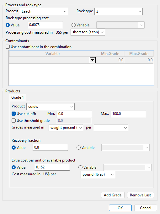
Select
 in the Combination Details grid to open the dialog in which to define the parameters for the combination.
-
If Use multiple product/process/rock type method is selected on the Financials pane, select the process identifier and rock type identifier from the Process and Rock type drop-down lists that will define the combination. The drop-down lists contain the process and rock identifiers defined in previous panes of the interface.
Note: If Use single product/process/rock type method is selected on the Financials pane, the interface assumes a default process method and rock type.
-
Define the overall cost to process a unit of feed material by selecting one of the following options for Rock type processing cost:
-
Value: Select this option to enter a constant value for the cost to process the rock type with the process for the combination.
-
Variable: Select this option to select a block model variable from the drop-down list that contains the cost to process the rock type with the process for the combination for each block.
-
-
Select the mass units in which the processing cost values are supplied from the Processing cost measured in drop-down list. This applies to both the constant or variable values for the Rock type processing cost.
-
Select the Use contaminant in the combination checkbox to restrict the material sent to the process based on the values in block model variables. If selected, only blocks where the values of the specified Variables are greater than or equal to the Min. Grade and less than or equal to the Max. Grade will be sent to the process. Select the block model variables from the Variable drop-down list and enter the minimum and maximum grade for the chosen variables in the Min. Grade and Max. Grade fields in the grid. Define more rows for additional contaminant variables as necessary.
Note: The same process-rock type pair can be set up with different processing parameters for high/low contaminant feed by creating multiple combinations
-
Select the applicable block model variable from the Product drop-down list, which contains variables corresponding to the product(s) defined on the Products pane to be processed.
-
Select the Use cut-off checkbox to ignore the product contents in a block based on the product grade. A minimum and a maximum cut-off grade must be specified in the Min. and Max. fields. If the grade of the block does not fall within the minimum and maximum grade, then that block cannot be processed under this combination.
-
Select the Use threshold grade checkbox to enter a threshold grade value below which the processing method is unable to recover. The feed grade of the process will be reduced by this amount when calculating the available product for this process to recover.
-
If Use cut-off and/or Use threshold grade is selected, specify the Grades measured in by selecting from the drop-down lists; if neither of these options were selected, this entry does not apply. Select the grade units for which cut-off and threshold values are expressed. Grade units can be selected using one of the two available direct grade units or by using a combination of mass units. The units should match those defined in the Products pane.
Threshold grade
Threshold grade is the grade of the material that goes to tailings or other type of processing residual after going through the mineral recovery/meturgical process. No process can recover 100% of in situ product, so this is what you cannot process.
Since this grade cannot be recovered, the grade available is the initial grade minus the one sent to tailings. If you assume there no loss, then just use 0.
If two blocks of grades 10 and 5 grade units are going to send 1 unit to the tailings, then from block 1 you will get 9 grade units and from the other you get 4.
Recovery is usually complex. Applying a percentage/factor assumes your recovery is linear and only based on the product grade. However as shown in this example, if you were to apply just a factor to different grade you could not handle a fixed grade in the material out of processing. So recovery is normally handled in advance of Pit Optimizer with a script, which may mean you should use 0 threshold if there is a block model variable handling all of that. The options there try to accommodate some scenarios without requiring a script to pre-calculate recovery, but is is not always possible.
-
Define the Recovery fraction to use with each block when processed. Select Value to enter a constant value or Variable to select a block model variable containing the fractional recovery value for each block from the drop-down list.
-
Define the Extra cost per unit of available product, which is the cost beyond the processing cost that must be accounted for. This is applied prior to any recovery function. Select Value to enter a constant value or Variable to select a block model variable from the drop-down list.
-
Select the mass units for which the Extra cost per unit of available product are supplied from the Cost measured in drop-down list. This applies for both the constant or variable values.
-
If Use multiple product/process/rock type method is selected on the Financials pane, you can click Add Grade to add a new product to the combination. You also have the option to click Remove Last to remove the last product from the combination.
-
Click OK to return to the main panel and save changes to the Combination Details grid. If Use multiple product/process/rock type method is selected on the Financials pane, add additional combinations as needed by clicking the ellipsis in the next row of the grid and repeating these steps to define parameters for a different process, rock type, and/or product combination.
Note: The same combination of rock type / process can be set up more than once, to handle things like alternate behaviours with contaminants or at high verses low head grades.
Tonnages
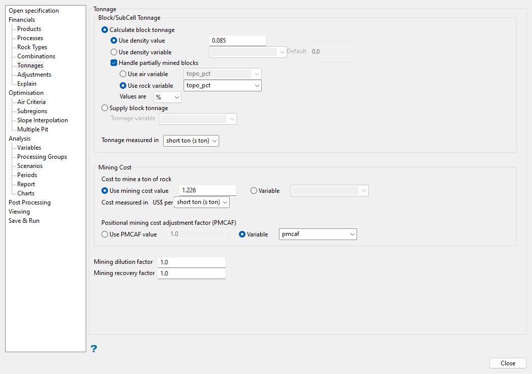
Use this pane to define the rock mass, choosing whether to calculate or supply block tonnage and specifying mining costs, mining dilution, and mining recovery.
Follow these steps:
-
Define the tonnage for each block with one of the following options:
-
Calculate block tonnage: Select this option if the tonnage has not previously been calculated in a block model variable. The optimiser will derive the block mass from a provided density value and the block volume.
-
Define the density of the material to be mined by either selecting Use density value and entering a constant value, or selecting Use density variable and choosing the block model variable in which density values are stored from the drop-down list. With the Use density variable option, you will also need to specify the Default value, which will take effect when no density value is present for a block.
-
Select the Handle partially mined blocks checkbox if the block model contains a variable with information about either the proportions or percentages of rock or air in each block, such as that determined for partially mined blocks with respect to an existing pit or topographic surface. Select either Use air variable or Use rock variable depending on the method used to define the partially mined blocks (e.g. via the Block > Manipulation > Mine... option). Select the block model variable that contains information about either the amount of air or rock in each block from the respective drop-down list and specify what the Values are (i.e. units) for the variable by selecting either percentages (%) or fractions (°/1) from the drop-down list.
Example: If the Use air variable option is selected with Values are set to percentages (%), then a value of
25in the variable means that 75% percent of the block's volume is rock.Note: You should not use Handle partially mined blocks if the block density is already reduced to account for this.
-
-
Supply block tonnage: Select this option if the block mass has already been calculated and stored in a block model variable. Select the block model variable that contains block tonnage from the Tonnage variable drop-down list.
-
-
Select the mass units in which the tonnage is measured in from the Tonnage measured in drop-down list. The specified mass units apply to both calculated and supplied block tonnage. In the case of calculated tonnage, the chosen units must correspond to the units of the density multiplied by the block volume units.
-
In the Mining Cost section, specify how the cost of mining each unit will be determined. Define the Cost to mine a ton of rock by selecting either Use mining cost value and entering a constant unit cost, or selecting Variable and choosing the block model variable that contains the unit cost for each block or sub-block from the drop-down list.
-
Select the mass units in which the mining cost is measured in from the Cost measured in drop-down list.
Note: Even if a cost of $0 is selected, units must be entered.
-
Define the Positional mining cost adjustment factor (PMCAF) that will be used to change the cost of mining the block due to its position in the mine.
Note: If the Variable selection for Cost to mine a ton of rock already accounts for block position, then there is no need for this factor. In this case, select Use PMCAF value and enter a value of
1.0.Select the Use PMCAF value option to enter a constant value to be applied to every block in the model regardless of the block position, essentially acting as a conventional mining cost adjustment factor. Alternatively, if the PMCAF has been determined and stored in a block model variable, select Variable to choose the block model variable that contains the PMCAF for each block from the drop-down list.
Example: If this factor should increase with depth, a variable in the block model should be populated with factors appropriate to the block depth in the pit design.
-
Enter the Mining dilution factor that will be applied to the total processing cost for the block. As this is a fractional value, no alteration will occur if a value of
1.0is entered. -
Enter the Mining recovery factor that will be applied to the total processing cost and the recovered product for the block. As this is a fractional value, no alteration will occur if a value of
1.0is entered.
Adjustments
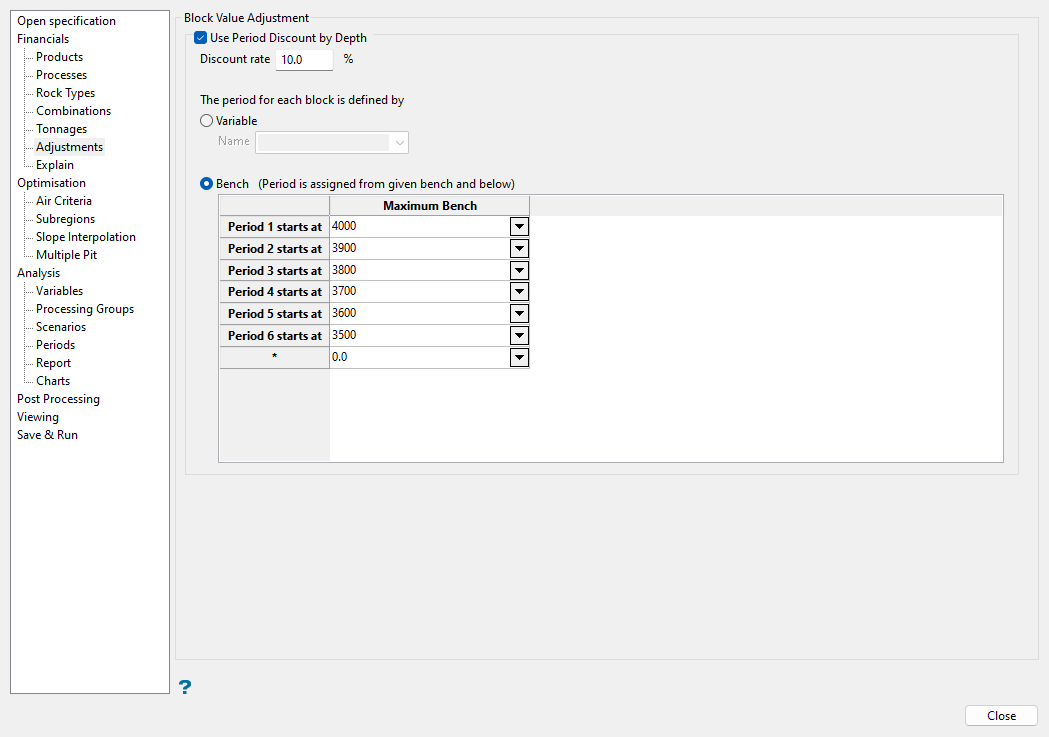
Use this pane to calculate a net present value (NPV) of each block based on the period in which the block will be mined. The adjustment process is iterative, as the exact mining sequence is not known when initially running the pit optimisation. As more information is made available, the adjustments will become more exact and meaningful to the final pit limits.
Follow these steps:
-
Select the Use Period Discount by Depth checkbox to enable the options in the pane to define the discount rate and period. If this checkbox is not selected, none of the options in this pane will be available.
Note: By adjusting the value of the block by period, a more realistic pit outline can be determined. However, these discounts are not used by the analysis functionality of the interface.
-
Enter the Discount rate, which varies by company and commodity.
Example: Entering 10% would mean each subsequent period is discounted by 10% of the previous amount (i.e. 90% -> 81% etc.)
-
Specify the method that The period for each block is defined by with either Variable or Bench.
-
Variable: Select this option if the period in which a block is to be mined can be defined by a block variable. Choose the block model variable that contains the period for each block from the Name drop-down list. The values stored in the variable should be whole numbers beginning at one (1) and increasing through the life of the mine.
Tip: If a bench will not be completely mined in a single period, it is best to use a block variable to define the period.
-
Bench: Select this option to define the periods by the mining bench. Choose a value from the first Maximum Bench drop-down list in the grid to define the beginning of the period, then select the next value in the second drop-down list to define the end of that period and the start of the next, and so on.
-
Explain
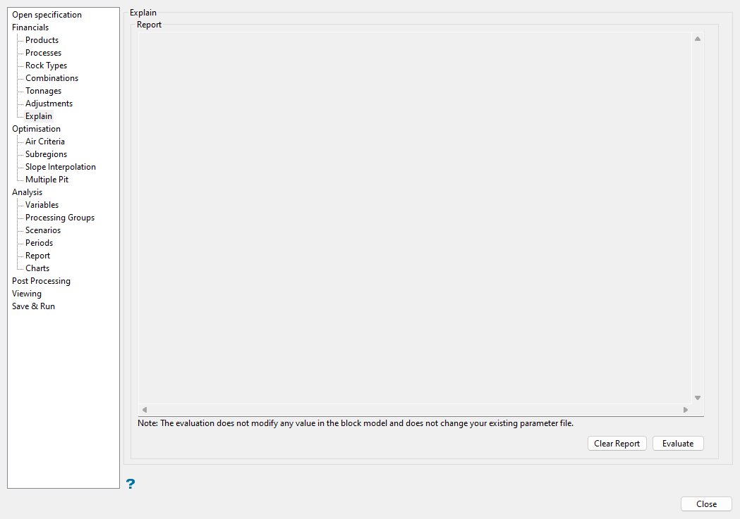
Use this pane to query blocks in a loaded block model and report details to gain a better understanding of how the optimiser is calculating the block values based on the current inputs in the interface.
Follow these steps:
-
Ensure that the blocks of interest have been loaded in the Vulcan workspace in an orientation where they can be selected.
-
Click the Evaluate button at the bottom of the pane. The interface will be collapsed and you will be prompted to indicate the block of interest in the Vulcan workspace.
-
Click on a loaded block. You will be returned to the main interface and the Report section of the pane will display all costs and revenues for the selected block. If adjustments were used, the adjusted value will also be present on the pane.
Tip: Using Snap To Objects mode or viewing in sections may be useful when selecting blocks.
Optimisation
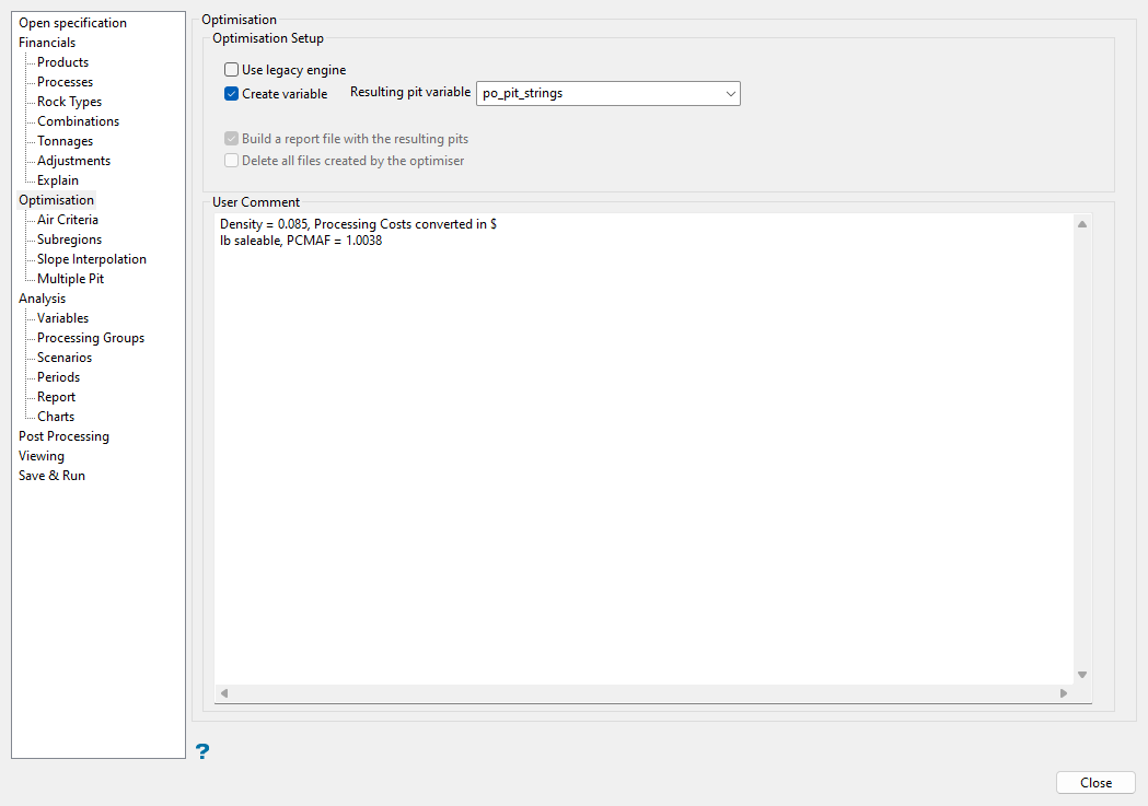
Use this pane to nominate the variable in which the optimisation results will be saved and define other optimisation setup preferences.
Follow these steps:
-
Select the Use legacy engine checkbox to use the traditional Lerchs and Grossman algorithm. There are two engines to solve the optimisation problems, each of which will produce the same result. If this checkbox is not selected, the updated, faster optimisation method is used.
-
Select the Create variable checkbox to create the Resulting pit variable in the block model if it is absent when the run is performed. Specify the Resulting pit variable in which the optimisation results will be stored by selecting an existing block model variable from the drop-down list, or enter a name for a new variable. This variable is typically an integer type block variable, and defines the optimal pit limits once the optimisation is completed.
Optimisation results are the number of the nested pit in which the block is contained. The following diagram demonstrates how the results are stored after the optimisation is performed and after fixing the air blocks.
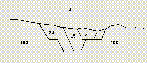
Figure 1 : Block Model After Pit Optimisation
-
If the Use legacy engine checkbox is selected, you will have the option to save an ASCII report file (
.respit) with the resulting pits from the optimisation by selecting the Build a report file with the resulting pits checkbox, which will be named after the optimisation parameters file (.opf). This file contains plan view maps of the resulting pits as ASCII art.Note: This option is not available if the Push-Relabel method is used.
Files outlining the optimisation process (
.log) as well as which pits were created and the factors used when multiple pits are considered (.fpp) are generated by default with the legacy engine, which can be viewed in a text editor. If these temporary files are not needed, select the Delete all files created by the optimiser checkbox, which is generally recommended. -
Enter a User Comment to aid in identifying the particular set of optimisation parameters, as desired.
Optimiser Criteria
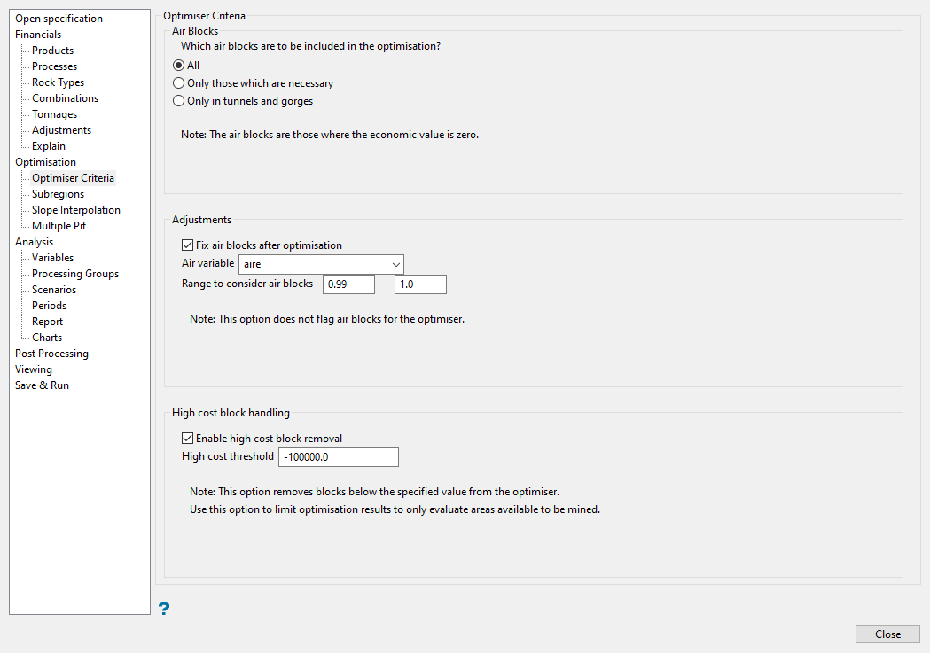
Use this pane to define the air blocks (i.e. those where the economic value is zero) to be considered during the optimisation and analysis. The optimiser uses air blocks to determine where the pit fits into the topographic surface. Without defined air blocks, the pit will extend to the top of the block model extents without considering the topographic surface.
Follow these steps:
-
Select one of the options below for Which air blocks are to be included in the optimisation?:
-
All: Select this option to consider all of the air blocks inside the block model. This is the default method and is recommended for very irregular topographic surfaces. However, it may cause the program to use excessive resources.
-
Only those which are necessary: Select this option to consider only air blocks that could have an influence inside the feasible pit. This method includes only air blocks that could influence the pit shape omitting all unnecessary air blocks.
-
Only in tunnels and gorges: Select this option to considers only the air blocks located in caves, tunnels, or gorges. This method is recommended for relatively flat surfaces. It uses only air blocks with rock above.
-
-
Select the Fix air blocks after optimisation checkbox to change the values of the resulting pit variable for air blocks. When contouring the results, the resulting lines will be adjusted automatically to the topography. If this checkbox is selected, you will need to choose the block model variable that defines the topography from the Air variable drop-down list and specify the Range to consider air blocks by entering a lower and upper bound of the value in the nominated variable to be considered as air.
Example: If you choose a block model variable that contains density values to define air blocks, then the range could be entered from
0.0to0.0. If the percentage of air was calculated in a block model variable, then a range from90to100could be entered, indicating that a block with over 90 percent air is considered to be an air block for contouring purposes. -
Select Enable high cost block removal to disallow mining block below the threshold value. You will need to set the High cost threshold value.
TipTip: When running the block calculation script (bcf) to flag the blocks that the Pit Optimiser will use, only flag blocks that are below your topographic surface. This will prevent blocks above the topographic surface from being part of the optimisation process even if this option is not enabled.
Keep in mind:
-
Flagging your model top to bottom with a highly negative value will result in air blocks being handled differently. This is because an air block is a block with a value of 0, so any block that does not have a value of 0 will not be considered air. For example, if block_value = tonnage * (-100000000000000) and you have no tonnes, the results might not be what you expect.
-
Enable the option to exclude high cost blocks to remove any block from the optimization below the user specified threshold.
-
When assigning negative values based on tonnage, keep in mind that blocks near topography can have very little tonnage and may not yield a cost beneath the threshold value.
-
Subregions
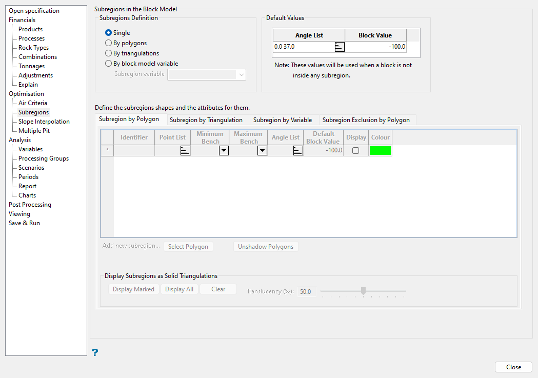
Use this pane to define spatial subregions with different pit slope requirements.
Follow these steps:
-
Select a Subregions Definition method from the following options:
-
Single: Select this option if only a single region is to used, that is, no subregions.
-
By polygons: Select this option if the regions are defined by 2D polygons with vertical influence defined by bench extents.
-
By triangulations: Select this option if the regions are defined using solid triangulations.
-
By block model variable: Select this option if the regions are defined by values stored in a block model variable. You will need to select the block model variable containing the subregion identifier values from the Subregion variable drop-down list.
Note: Only one method may be used in a single optimisation run.
-
-
Set the Default Values for the slope angle requirements and the default economic value used for blocks not identified as part of a subregion by defining the Angle List and Block Value fields in the grid, respectively.
Note: These defaults are used for all blocks if the Single subregion option is selected.
-
Populate the Angle List by selecting
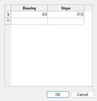
 to display the following dialog, where an irregular cone shape is defined that represents the default pit slope angle requirements. Enter the Bearing to define the orientation at which the slope angle corresponds, and enter the associated slope angle in the Slope field. Populate additional rows as needed to define slope angles for different bearings and click OK to save entries and return to the main panel.
Tip: Refer to the Slope Interpolation pane to define how the pit slope will change from one bearing to another.
-
Enter the Block Value used to adjust the economic value of all blocks found to be missing volume. This is the case when blocks have been deleted from the block model. If block model blocks (or sub-blocks) do not occupy the entire optimisation block volume, the absolute value of this value will be subtracted from the economic value of the optimisation block proportionally to the missing volume.
Note: Deleting air blocks is a fairly common practice. In that case, the negative value will apply to every deleted air block.
-
-
Define subregion shapes and the associated attributes with the respective grids in the tabs present in the pane for subregions characterised by polygons, triangulations, or variables, depending on your selected method for the Subregions Definition.
Note: You can apply Subregion Exclusion by Polygon definitions for all subregions definition methods.
 Subregion by Polygon
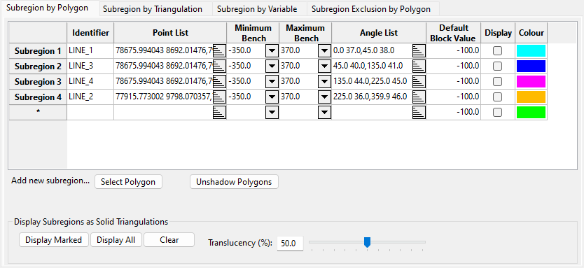
If By polygons is selected for the Subregions Definition method, use this grid to identify the polygons of interest, with the vertical influence set by selecting minimum and maximum bench extents, and define slope angles and default economic values for the resulting subregions. Additional options below the grid area allow you to display the defined subregions.
-
Ensure that any polygons that will be used to define subregions are loaded to the Vulcan workspace.
-
Click the Select Polygon button below the grid and pick the desired polygon from the Vulcan workspace. The Identifier matching the polygon object name and the Colour of the selected object will be added to the grid, and the X and Y index coordinates defining the polygon will be loaded in the Point List field.
Tip: Edit the Identifier as needed to provide an informative name for the zone defined by the polygon. You can also click
 in the Point List cell to open the dialog in which you can review the loaded points.
 -
Select the Minimum Bench and the Maximum Bench from the drop-down lists to define the vertical influence zone of the polygon for the subregion. The lower limit of the defined subregion is the same as the minimum bench elevation, and the upper limit is the maximum bench elevation plus the vertical size of the optimiser block model, that is, after any dynamic re-blocking.
-
Click
 in the Angle List cell to open the dialog in which to define the slope angle requirements of the subregion by entering Bearing and Slope values, in the same way as the Angle List is defined above in the Default Values section of the pane.
 -
Enter the Default Block Value that will be assigned to each block of the optimiser block model size when the block volume is missing. If the missing part is smaller than the optimiser block model size, then the value is assigned to the block proportional to the volume missing.
-
Click the Display checkbox to mark the subregion to be displayed as a solid triangulation on-screen when the Display Marked button is clicked at the bottom of the pane. The subregion triangulations are formed by projecting the polygon between the minimum and maximum bench extents. The triangulation colour is defined through the Colour field in the grid, which can be changed from the colour associated with the selected polygon by clicking the Colour cell and choosing from the colour palette table. Adjust the Translucency of the triangulations as desired before displaying them by entering a percentage or moving the slider bar.
You can also click Display All to display all of the defined subregions as solid triangulations on-screen, regardless of if the Display checkbox is selected in the grid, or Clear to remove the triangulations currently displayed.
Note: When the subregion triangulations are displayed, they are saved to the current working directory with triangulation file names matching the Identifier field.
-
If you would like to create a new subregion based on a polygon, start a new row in the grid and repeat these steps. You can click Unshadow Polygons to make previously selected polygons that have been greyed out (i.e. disabled) available for selection again for cases when a polygon is needed more than once to define subregions.
 Subregion by Triangulation
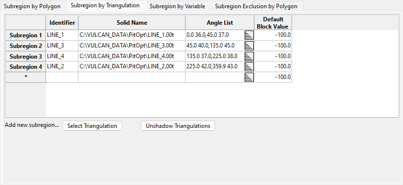
If By triangulations is selected for the Subregions Definition method, use this grid to identify triangulations of interest and define slope angles and default economic values for the resulting subregions.
-
Enter an Identifier that provides an informative name for the zone defined by the triangulation.
-
Nominate the solid triangulation by which to define the subregion in the Solid Name field. Select a triangulation file from the drop-down list in the cell, which contains all triangulations in the current working directory, or click
 to navigate to another folder location.
 Alternatively, click the Select Triangulation button below the grid to pick the desired triangulation from those loaded to the Vulcan workspace. With this method, the Identifier matching the triangulation name will be added to the grid.
-
Click
 in the Angle List cell to open the dialog in which to define the slope angle requirements of the subregion by entering Bearing and Slope values, in the same way as the Angle List is defined above in the Default Values section of the pane.
 -
Enter the Default Block Value that will be assigned to each block of the optimiser block model size when the block volume is missing. If the missing part is smaller than the optimiser block model size, then the value is assigned to the block proportional to the volume missing.
-
If you would like to create a new subregion based on a triangulation, start a new row in the grid and repeat these steps. You can click Unshadow Triangulations to make previously selected triangulations that have been greyed out on-screen (i.e. disabled) available for selection again.
 Subregion by Variable
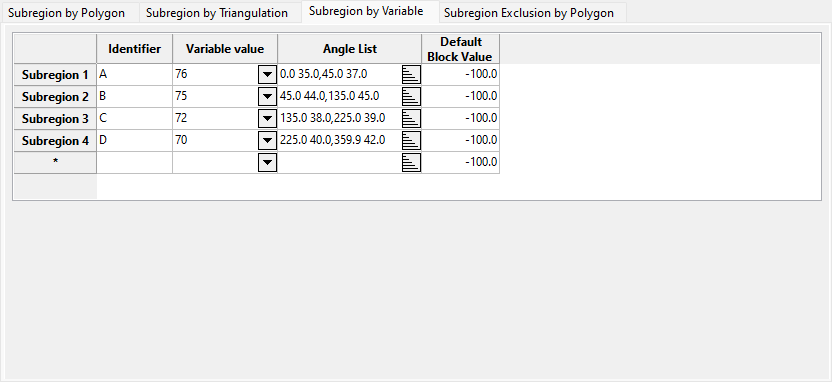
If By block model variable is selected for the Subregions Definition method, use this grid to identify values of interest from a block model variable and define slope angles and default economic values for the resulting subregions.
-
Enter an Identifier that provides an informative name for the zone defined by the variable value.
-
Specify the Variable value by which to define the subregion by entering the value of interest. If the variable is alphanumeric, you can select entries from the drop-down list, which contains all of the subregion identifier values present in the block model variable nominated for the Subregion variable under the Subregions Definition section.
-
Click
 in the Angle List cell to open the dialog in which to define the slope angle requirements of the subregion by entering Bearing and Slope values, in the same way as the Angle List is defined above in the Default Values section of the pane.
 -
Enter the Default Block Value that will be assigned to each block of the optimiser block model size when the block volume is missing. If the missing part is smaller than the optimiser block model size, then the value is assigned to the block proportional to the volume missing.
-
If you would like to create a new subregion based on a variable value, start a new row in the grid and repeat these steps.
 Subregion Exclusion by Polygon
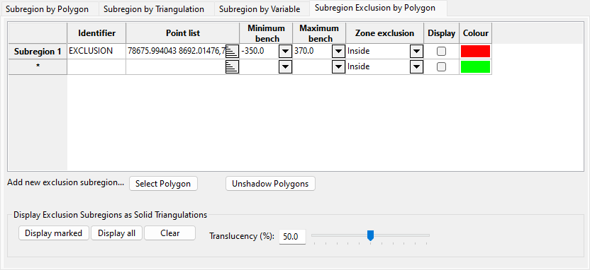
This grid is available for all Subregions Definition methods and allows you to exclude the zone inside or outside of subregions defined by polygons of interest, with the vertical influence set by selecting minimum and maximum bench extents, from the pit limits determined by the optimiser (i.e. exclusion zone will not be mined). Additional options below the grid area allow you to display the defined subregions.
-
Ensure that any polygons that will be used to define subregions are loaded to the Vulcan workspace.
-
Click the Select Polygon button below the grid and pick the desired polygon from the Vulcan workspace. The Identifier matching the polygon object name and the Colour of the selected object will be added to the grid, and the X and Y index coordinates defining the polygon will be loaded in the Point List field.
Tip: Edit the Identifier as needed to provide an informative name for the zone defined by the polygon. You can also click
 in the Point List cell to open the dialog in which you can review the loaded points.
 -
Select the Minimum Bench and the Maximum Bench from the drop-down lists to define the vertical influence zone of the polygon for the subregion. The lower limit of the defined subregion is the same as the minimum bench elevation, and the upper limit is the maximum bench elevation plus the vertical size of the optimiser block model, that is, after any dynamic re-blocking.
-
Specify whether the optimiser should exclude the zone inside or outside of the defined subregion by selecting Inside or Outside from the Zone exclusion drop-down list.
-
Click the Display checkbox to mark the subregion to be displayed as a solid triangulation on-screen when the Display Marked button is clicked at the bottom of the pane. The subregion triangulations are formed by projecting the polygon between the minimum and maximum bench extents. The triangulation colour is defined through the Colour field in the grid, which can be changed from the colour associated with the selected polygon by clicking the Colour cell and choosing from the colour palette table. Adjust the Translucency of the triangulations as desired before displaying them by entering a percentage or moving the slider bar.
You can also click Display All to display all of the defined subregions as solid triangulations on-screen, regardless of if the Display checkbox is selected in the grid, or Clear to remove the triangulations currently displayed.
Note: When the subregion triangulations are displayed, they are saved to the current working directory with triangulation file names matching the Identifier field.
-
If you would like to create a new subregion for exclusion based on a polygon, start a new row in the grid and repeat these steps. You can click Unshadow Polygons to make previously selected polygons that have been greyed out (i.e. disabled) available for selection again for cases when a polygon is needed more than once to define subregions.
-
Slope Interpolation
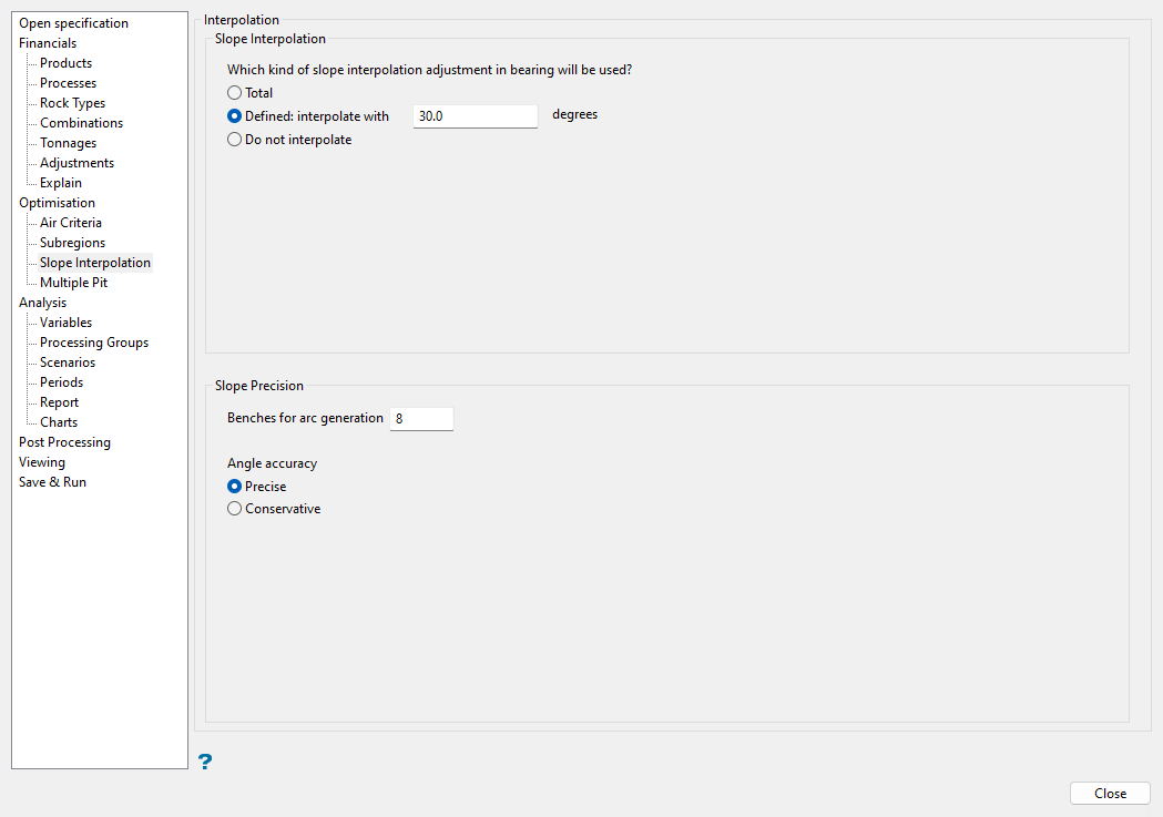
Use this pane to specify how the optimiser will interpolate between slope angles set for specific bearings, as defined on the Subregions pane. The precision of the slope angle used to determine prerequisite mining blocks is also defined in this pane.
Follow these steps:
-
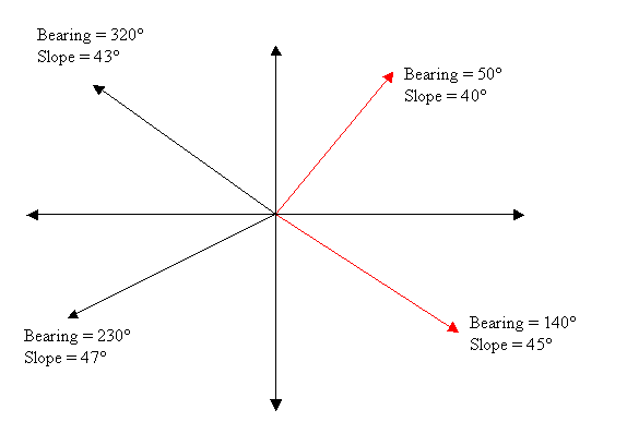
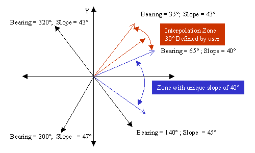
Select one of the options below for Which kind of slope interpolation adjustment in bearing will be used? and see the annotations added to the following base diagram to further describe each option. The base diagram below demonstrates four slope angle bearing definitions made in the Angle List area of the Subregions pane:
-
Total: Select this option to use the entire zone between defined bearings to interpolate the pit slope angle. The pit slope angle set for each bearing in the Subregions pane is used only at the starting azimuth.
-
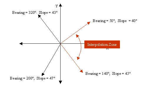
Defined: Select this option to define a range (between 15° and 40°) to interpolate within by entering an angle in the interpolate with <##> degrees field. The resulting interpolation zone will be centred around the defined bearings. The beginning of each interpolation zone starts at the previous slope definition, and the end of each interpolation zone matches the defined slope angle for the respective bearing. In the example in the following diagram, 30° was used to perform the interpolation.
-
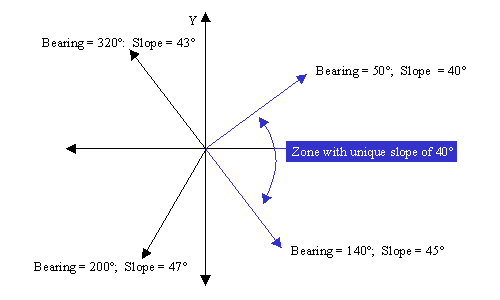
Do not interpolate: Select this option to maintain the slope angle for the defined bearing up to the next defined bearing. In the example in the following diagram, the result shows a 40° slope angle between azimuths of 50° and 139.999°.
-
-
Enter the number of benches that will be used to define the geometrical constraints for each subregion in the Benches for arc generation field. The more benches that you specify, the more closely the average slope will match the defined slope angle and the longer the optimisation will take.
Important: Using more benches than exist in the model will cause the optimiser to give invalid results.
You may need to iterate to find the best solution, but as a starting value we suggest using eight times the largest of the two horizontal dimensions of a block divided by the height of a block. That is:
[Max(Bx,By)*8]/BZWhere:
BX is the X dimension of a block
BY is the Y dimension of a block
BZ is the Z dimension of a block
With typical slopes of 40 to 50 degrees from the horizontal, this will usually give an average slope error on the order of one degree.
-
Define the Angle accuracy method by selecting one of the following options:
-
Precise: Select this option to include blocks as predecessors to a given block if the angle between them is larger than or matches the required slope angle within a tolerance of 0.001 degrees.
-
Conservative: Select this option to include blocks as predecessors to a given block if the angle between them is larger than or matches the required slope angle within a tolerance of 0.5 degrees. This option will include more blocks as predecessors than the Precise option and will result in pit slopes that are slightly more conservative than the defined slope angles in the Subregions pane.
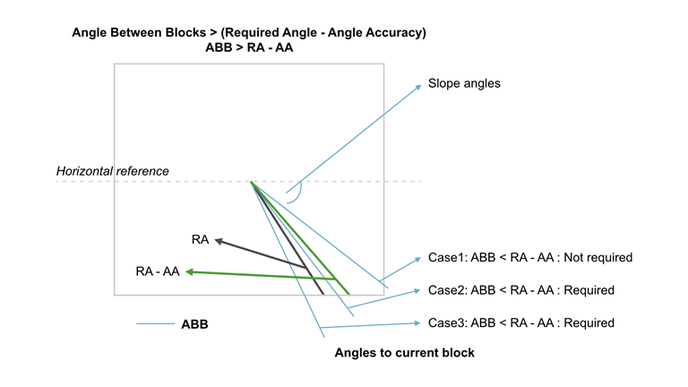
NoteSince angles can only be achieved discretely, the slope angle cannot be reached exactly at all block locations. In order to generate block precedence relationships for a given block, blocks in layers above the current block are considered. For each pair of blocks evaluated, the angle between the blocks is computed. If the slope angle between the current block and one in a layer above it is higher than the required slope, also considering the tolerance from the selected angle accuracy method, then the block in the overlying layer is a prerequisite to the current block being mined. That is, a block is considered a prerequisite of the current block if:
Angle Between Blocks > (Required Angle - Angle Accuracy)Only the first benches for arch generation layers are considered in this evaluation.
The diagram below shows three different cases for angles between blocks with respect to the required slope angle and the angle accuracy, and if the upper block in each case is a required prerequisite to the current block being mined.
-
Multiple Pit
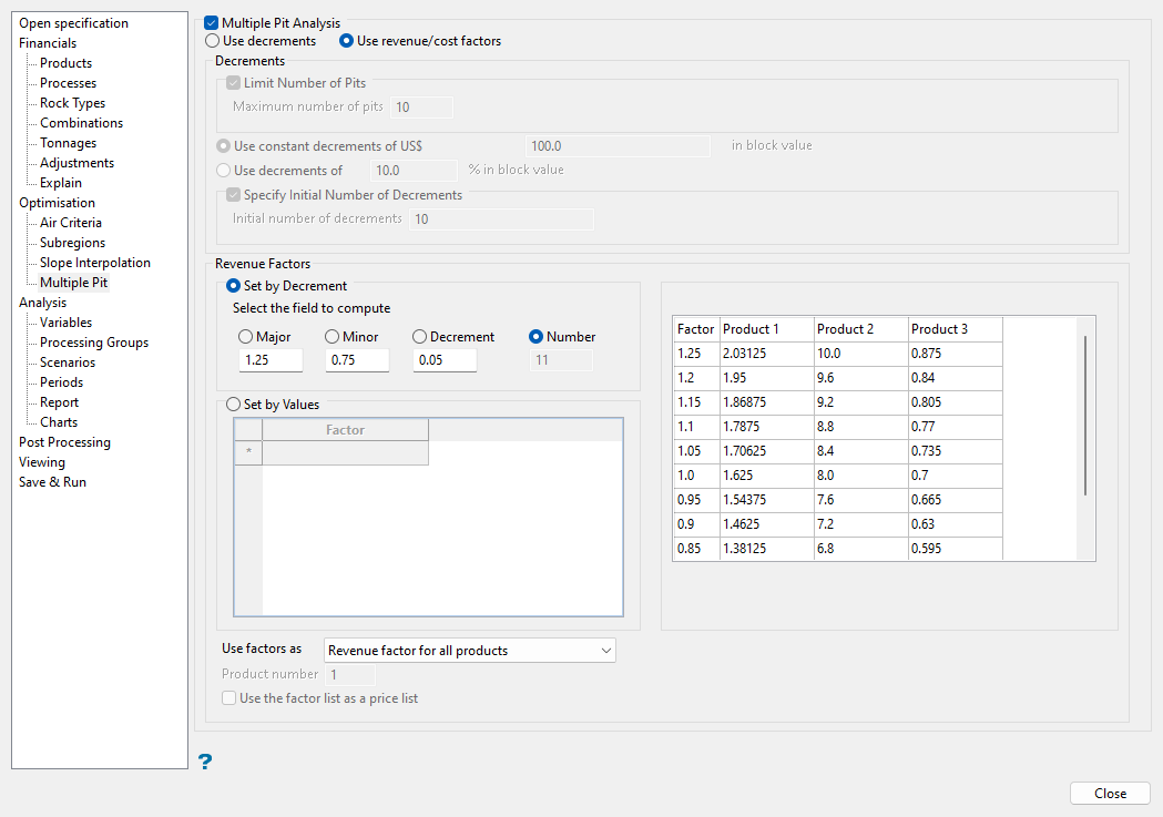
Use this pane to define parameters used to create and optimise multiple pits and perform sensitivity analysis studies.
Follow these steps:
-
Select the Multiple Pit Analysis checkbox to active the options in this pane. If this option is not checked, then either the economic block value or the initial product prices will define the scenario used to determine the only pit.
-
Select whether to Use decrements to alter the economic value of blocks by a constant value or percentage, or Use revenue/cost factors to have more control over altering the economic value of blocks when analysing multiple pits:
Note: The Use revenue/cost factors option is only available if Calculate Economic Value is selected in the Financials pane.
-
Use decrements: Select this option to reduce the economic value of the ore blocks by a fixed amount or percentage of block value for each successive run.
-
Select the Limit Number of Pits checkbox to enter a value for the Maximum number of pits to be generated by the optimiser. This is most necessary when decrements are applied as percentages.
-
Select either the option to Use constant decrements and enter the fixed amount in block value to decrement the economic value of ore blocks for each new trial, or Use decrements of and enter a percentage in block value to decrement the economic value of the current ore blocks in a fractional fashion for each new trial. Waste block values are not changed with either of these options.
-
Select the Specify Initial Number of Decrements checkbox to enter a value in the Initial number of decrements field, which may be desired if the Push-Relabel algorithm is being used for the optimisation. This will be used to determine the economic value of pit 1.
Note: This option is only available if the Use legacy engine checkbox is not selected on the Optimisation pane.
-
-
Use revenue/cost factors: Select this option to alter the way the block value itself is obtained. Using a set of factors, either prices or costs are changed to obtain a different economic value for each block.
-
Select either Set by Decrement to define the revenue or cost factors by entering values for the Major (maximum factor), Minor (minimum factor), Decrement (factor spacing), and Number (number of factors) fields—except for the field that is selected to be computed—to generate evenly spaced factors, or Set by Values to manually specify the factors in the grid that will be applied to prices or costs, which do not need to be evenly spaced.
-
Select one of the options below from the Use factors as drop-down list to indicate how the revenue/cost factors are used to control the parameterisation of the economic value:
-
Revenue factor for all products: Use this option to compute the ore value for each product by applying the set factors to the revenue for all products in each block:
Base price * Revenue factor -
Revenue factor for one product: Use this option to compute the ore value for the specified product number by applying the set factors to the revenue of the selected product in each block:
Base price * Revenue factorWith this option, you will need to specify the Product number to modify using the revenue factors, corresponding to the product order listed in the Products pane. Select the Use the factor list as a price list checkbox to use the defined factors directly as prices for the specified element, rather than multiplying the base price by the factor.
Note: All other products will be remain with a single base price, as defined through the Products pane.
-
Cost factor for all combinations' process cost: Select this option if you want to apply the factors to the process cost for all combinations. The process cost will be changed by multiplying the reference process cost, which was defined through the Combinations pane, by the factors specified here.
-
Cost factor for all products' selling cost: Select this option if you want to apply the factors to the selling cost for all products. The selling cost will be changed by multiplying the reference selling cost, which was defined through the Products pane, by the factors specified here.
-
Cost factor for mining cost: Select this option if you want to apply the factors to the mining cost for all blocks. The mining cost will be changed by multiplying the reference mining cost, which was defined through the Tonnages pane, by the factors specified here.
-
-
Based on your selections, review the resulting factors and prices/costs in the summary grid on the right side of the pane.
-
-
Analysis
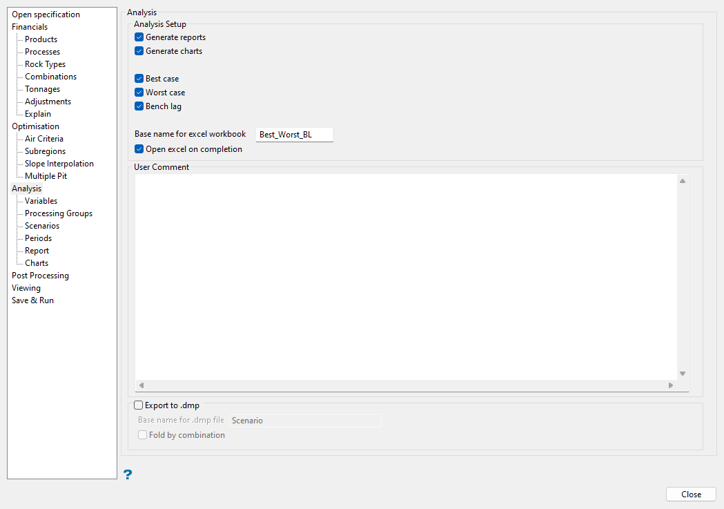
Use this pane to make selections for creating reports and charts based on optimisation results.
Follow these steps:
-
Select the Generate reports and/or Generate charts checkboxes to create tabulated analysis reports and charts, respectively, based on the pits generated in the optimisation process. The analysis will be performed on results stored in the Pit variable specified in the Variables pane. Configure the details of the applicable analysis outputs in the Report and Charts panes.
-
If you elected to generate reports or charts, the following options will become available to include in the analysis outputs and define how the blocks will be sequenced according to the nested pit information in the block model:
-
Best case: This method will fully mine each pit shell top to bottom before proceeding to the next pit shell.
-
Worst case: This method mines each bench out by increasing pit shell order, that is, the largest pit shell’s blocks from the previous bench must be fully mined before proceeding the first pit shell’s blocks in the next bench.
-
Bench lag: This method allows you to specify a maximum bench separation between consecutive pit shells. The mining sequence will force the blocks from the next pit shell to be mined with the current pit shell if the bench separation between the consecutive pit shells is going to be greater than the maximum allowable bench lag. The lag separation is defined through the Variables pane.
-
-
After selecting the Best case, Worst case, and/or Bench lag option, you will be able to enter the Base name for excel workbook to be used as a prefix for the Excel file names generated from the analysis. Select the Open excel on completion checkbox to open the output file in Excel after the analysis is run. Add a User Comment as desired to include extra information for future reference regarding the analysis parameters.
-
Select the Export to .dmp checkbox to analysis output results to
.dmpfiles as well as.chronos_idsfiles that can be imported into Excel for manipulation and high-level scheduling. Enter the Base name for .dmp file to be used as a prefix for the generated files. Leave the Fold by combination checkbox unselected to report each combination as a separate key.
Variables
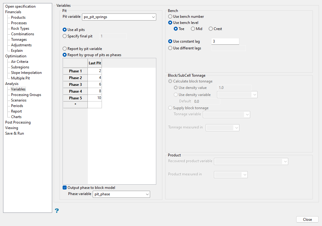
Use this pane to configure how the optimisation pit results stored in the nominated block model variable will be presented in the reports and charts.
Follow these steps:
-
Select the block model variable that contains the nested pits generated from the optimisation process from the Pit variable drop-down list. The definition of nested pits stored in this variable can be used directly or pits can be grouped as phases with the options in this pane.
Note: Failure to select the same variable as specified on the Optimisation pane can result in incorrect information being reported.
-
If Multiple Pit Analysis is enabled on the Multiple Pit pane, specify the pits to include in the analysis by selecting either Use all pits to consider all the nested pits found in the pit variable, or Specify final pit to exclude pit numbers from the analysis that are higher than the entered value and consider the specified value as the final pit number.
Note: When selecting which pits to use in the analysis, it is important to note that pit 1 is always the smallest pit. Pit numbers will increase as pit size increases. These numbers correspond to the number of factors or decrements defined in the Multiple Pit pane.
-
If Multiple Pit Analysis is enabled on the Multiple Pit pane, select from the following options to define how to report the pits:
-
Report by pit variable: Select this option to perform the analysis per pit with the pit values as they are stored in the block model variable.
-
Report by group of pits as phases: Select this option to group pits together for the analysis and replace the original pit numbering in the pit variable with the group definition. In reports and charts, the name
Pitwill be used to refer to the phase groups.-
Define pit phase groups in the grid by entering the Last Pit value to be included in each phase. Each Last Pit entry in the grid must be a value greater than the previous entry. Each phase includes pit values greater than the previous Last Pit entry up to and including the current Last Pit.
-
Select the Output phase to block model checkbox to output the phases to a block model variable, and select the desired Phase variable from the drop-down list.
-
-
-
Select either Use bench number to report benches as consecutive integer numbers from bottom up, or Use bench level to report benches by elevation and specify whether to use the bench Toe, Mid, or Crest elevation. Bench elevation and locations are related to the optimiser block model parent size.
-
If Bench lag is selected on the Analysis pane, you will have the option to Use constant lag and enter the same bench lag for all the pits/phases in the analysis, or Use different lags to define different bench lags for the pits/phases in the analysis.
Example: An entry of
5 p4:7in the Use different lags field indicates a lag of 5 for the first pits/phases, then at pit or phase 4 (depending on the report by selection) the lag changes to 7. The syntax for this field requires that a constant lag value be entered at the beginning and changes must be entered sequentially. A change can only occur for a pit/phase with a number higher than the previous change. -
If Supply Economic Value is selected on the Financials pane, you will need to define parameters to report tonnage in this pane by selecting Calculate block tonnage or Supply block tonnage, since the optimiser did not require block tonnage previously.
Note: When Calculate Economic Value is used, the optimiser reuses the tonnages calculated during optimisation.
-
Calculate block tonnage: Select this option if the tonnage has not previously been calculated in a block model variable. The block mass will be derived from a density value and the block volume.
You will need to define the density of the material to be mined by either selecting Use density value and entering a constant value, or selecting Use density variable and choosing the block model variable in which density values are stored from the drop-down list. With the Use density variable option, you will also need to specify the Default value, which will take effect when no density value is present for a block.
-
Supply block tonnage: Select this option if the block mass has already been calculated and stored in a block model variable, and select the Tonnage variable that contains block tonnage from the drop-down list.
For either calculated or supplied block tonnage values, you will need to specify the mass units by selecting from the Tonnage measured in drop-down list. In the case of calculated tonnage, the chosen mass units must correspond to the units of the density multiplied by the block volume units.
-
-
If Supply Economic Value is selected on the Financials pane, you will need to populate fields in this pane in order to report product units, since the optimiser did not require a definition of products previously. Select the Recovered product variable from the drop-down list, and specify the product units by selecting from the options in the Product measured in drop-down list.
Processing Groups
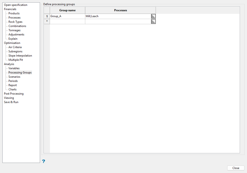
Use this pane to create processing groups that can be used in the Scenarios pane to evaluate and report on combined process capacities per period rather than target individual process capacities.
Note: The options in this pane will only be available if Use multiple product/process/rock type method is selected on the Financials pane. You will also need to populate the Processes pane so that defined process names can be selected when creating processing groups in this pane.
Follow these steps:
-
Enter a unique name for each processing group in the Group name column.
-
Click
 in the Processes column to open the dialog used to add processes to each group. Select the processes to be included in the group from the drop-down lists in the dialog's grid and click OK to return to the main panel.
Scenarios
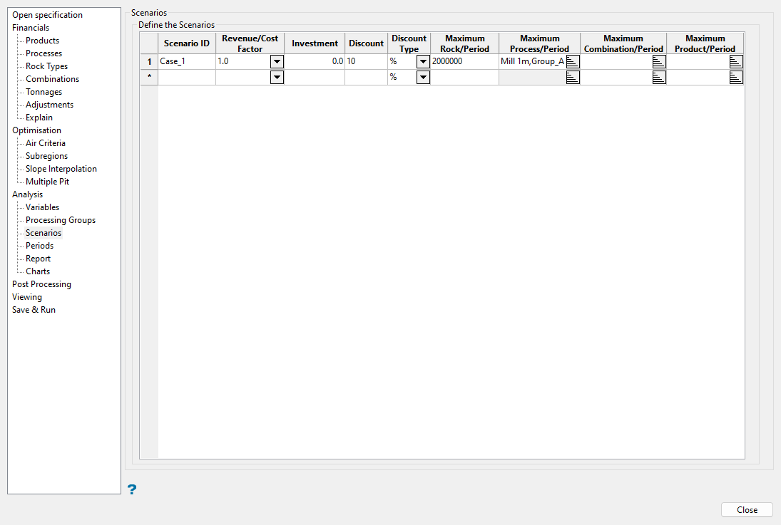
Use this pane to define constraints used in analysis scenarios that establish periods as well as calculate material movements and cash flows. Analysis results for each scenario are saved to a separate Excel file.
Follow these steps:
-
Enter a unique name for each Scenario ID, which will be used to identify scenarios of interest in the Periods pane and also used as a suffix for the Excel file names.
Note: If you open a specification file created from an older version of Vulcan, default scenario IDs may be assigned in the current interface.
-
Select the Revenue/Cost Factor you want to use for the scenario from the drop-down list, which contains factors defined in the Multiple Pit pane. This factor is applied to the calculated financials in the analysis, but does not affect which blocks are selected for inclusion in the report based on the corresponding pit (this is controlled by the Specify final pit option in the Variables pane).
-
Enter the initial capital investment in the Investment field, which will be used to calculate cumulated cash flows for the project.
-
Enter the Discount rate to be used for determining the discounted cash flow or net present value cash flow for the project. The discount rate is applied to the first year.
Example: If 5% is entered, the first year’s result will be reduced by 95%.
-
Select a Discount Type of either a percentage (%) or fraction (°/1) from the drop-down list based on the units applicable for the value entered in the Discount field.
-
Define the maximum rock movement—ore and waste—that can be achieved in each period in the Maximum Rock/Period field. The rock limit can be specified for different periods using the same syntax as the Discount field. See the following example entries for syntax that uses shortcuts for large numbers.
Syntax Explanation 5k p4:6kStart with 5,000, in period 4 increase to 6,000 500k p4:6ck p8:1mStart with 500,000, in period 4 increase to 600,000, and in period 8 increase to 1,000,000 1ckStarts with 100,000 without further changing the limit 1ccStarts with 10,000 without further changing the limit 5.1c1Starts with 5.1001 without further changing the limit (large number shortcuts after decimals places will be interpreted as the corresponding number of zeros after the decimal place) -
If Use multiple product/process/rock type method is selected on the Financials pane, you will have the option to click
 in the Maximum Process/Period field to open the dialog used to define process capacities. Select a Process from the drop-down list in the dialog's grid (which contains those defined in the Processes pane as well as any groups of processes defined in the Processing Groups pane, in addition to predefined Total Ore and Waste options) and enter a capacity specification for the process in each period in the Maximum Process/Period field. Different capacities can be specified for different periods for the process as well with syntax similar to that used for Maximum Rock/Period. Click OK to return to the main panel.
 The following entries define a maximum of 1,000,000 for the
Millprocess for all periods and a varying maximum forGroup_A, which is defined in the Processing Groups pane to include bothMillandLeachprocesses. The maximum forGroup_Ais defined as 1,500,000 for the first periods, changing to 2,000,000 at period 6.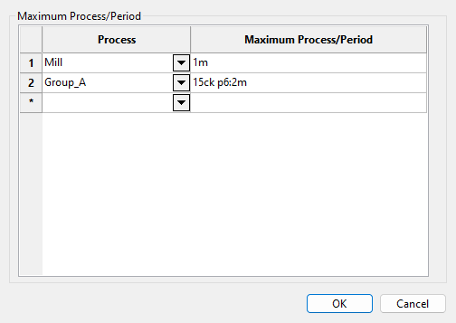
-
Click
 in the Maximum Combination/Period field to open the dialog used to define the capacity for a specific rock type in a process. Select a Combination from the drop-down list in the dialog's grid, which contains those defined in the Combinations pane, and enter a capacity specification for the combination in each period in the Maximum Combination/Period field. Different capacities can be specified for different periods for the combination as well with syntax similar to that used for Maximum Rock/Period. Click OK to return to the main panel.
 -
Click
 in the Maximum Product/Period field to open the dialog used to define the selling or production capacity for each product. Select a Product from the drop-down list in the dialog's grid, and enter a capacity specification in the Maximum Product/Period field. Different capacities can be specified for different periods for the product as well with syntax similar to that used for Maximum Rock/Period. Click OK to return to the main panel.
 -
Create more scenarios as needed by repeating these steps to populate additional rows in the grid.
Periods
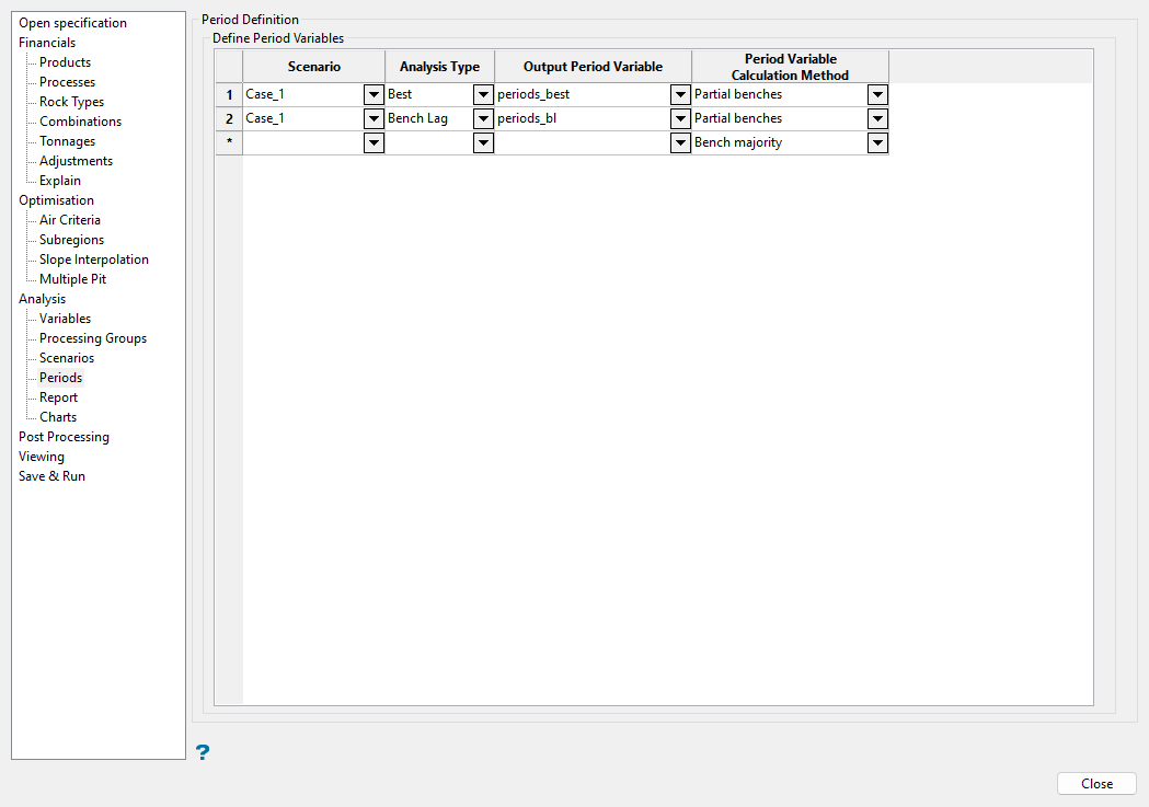
Use this pane to specify how the periods are written back into the block model.
Follow these steps:
-
Select the Scenario that the period data will be based on from the drop-down list, which contains all Scenario ID entries defined on the Scenarios pane.
-
Select the Analysis Type used to determine the block sequencing order for period determination from the drop-down list, which contains the methods enabled on the Analysis pane (i.e. Best case, Worst case, and/or Bench lag).
-
Specify the Output Period Variable that will be used to store the resulting period data by entering a new block model variable name or selecting an existing variable from the drop-down list.
-
Select the Period Variable Calculation Method used to flag which period a block exists within from the following options in the drop-down list:
-
Bench majority: Select this option to flag blocks within the same bench with the same period. If the period changes mid-bench, then the period that takes up the majority of the bench will determine the period for the whole bench.
-
Partial benches: Select this option to flag blocks with the periods of a bench based on what proportion of the bench is taken away in a particular period. Blocks are flagged with this method based on an area calculation.
Example: If 20% of a bench is taken away in period 1 and the rest of the bench is taken away in period 2, then 20% of the area of that bench will be flagged as being period 1 and the remaining 80% will be period 2.
-
First touch: Select this option to flag blocks within the same bench with the starting period.
-
Last touch: Select this option to flag blocks within the same bench with the ending period.
-
-
Create more periods as needed by repeating these steps to populate additional rows in the grid.
Report
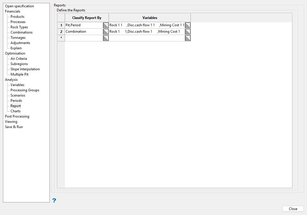
Use this pane to configure the different types of reports to save as tabs in an Excel file.
Note: Select Generate reports on the Analysis pane to activate the Report options.
Follow these steps:
-
Click
 in the Classify Report By field to open the dialog used to define how the analysis results for the blocks in the block model will be grouped in each report. Select one of the predefined classification fields from the Report Column drop-down list in the dialog's grid, which will designate the first column of the report to group results by, and make a selection for the report's second column if desired. Click OK to return to the main panel.
 Note: Each row in the Reports grid will generate a new report tab in the Excel spreadsheet, named with the report number followed by the Classify Report By entry.
The predefined report classification fields are listed below:
-
Period: Presents analysis results for blocks grouped by mining period.
-
Pit: Presents analysis results for blocks grouped by pit (or if the pits were grouped into phases in the Variables pane). Results for each pit include blocks that are flagged with smaller pits numbers as well, since the extents of the smaller pits are included in the extents of the larger pits (e.g. Pit 4 includes results for Pits 1 through 4).
Note: If Pit is selected as a report classification field, it must be specified as the first report column. If pit is specified as the second field, only values for the last pit will be exported.
-
PitIncrement: Presents analysis results for blocks grouped by each pit (or phase, if applicable) excluding the results of smaller pits included in the analysis that are encompassed within the pit of interest (i.e. not cumulative).
-
Process: Presents analysis results for blocks grouped by processing method.
-
RockType: Presents analysis results for blocks grouped by rock type.
-
Combination: Presents analysis results for blocks grouped by defined process, rock type, and product combinations.
-
Bench: Presents analysis results for blocks grouped by bench elevations.
-
-
Click
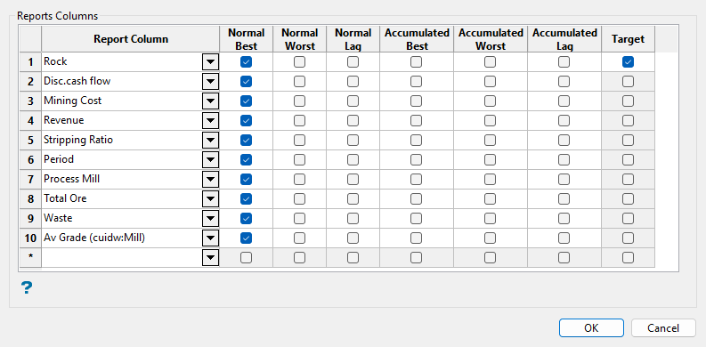
 in the Variables field to open the dialog used to define the variables to include for each report.
-
Select the variable to include in the report from the Report Column drop-down list. The variables will be ordered within the report based on the order in which they are selected in this grid.
-
Select the adjacent checkboxes for the analysis type to use for each variable. Depending on the sequencing methods specified in the Analysis pane, best, worst, and bench lag methods are available for accumulated quantities of the report column. Each checkbox selected will create a column in the report.
If reporting by period (i.e. Classify Report By is set to Period), and the variable selected for the Report Column is Rock, then selecting the Accumulated Best checkbox will present the cumulated rock tonnage extracted for each period in the report when the sequence method was best case.
If the Normal Worst checkbox is selected, then the partial tonnage for each period displays with the quantities corresponding to the worst case sequencing method.
-
Select the Target checkbox to report the target for the given report column variable if the variable is in the list for limiting capacities. Rock, Process, Product, and Combination can be used to specify limits. Only these columns will be available to display the targets when the limiting quantity for the column displays in the chart.
-
-
Create more reports as needed by repeating these steps to populate additional rows in the grid.
Charts
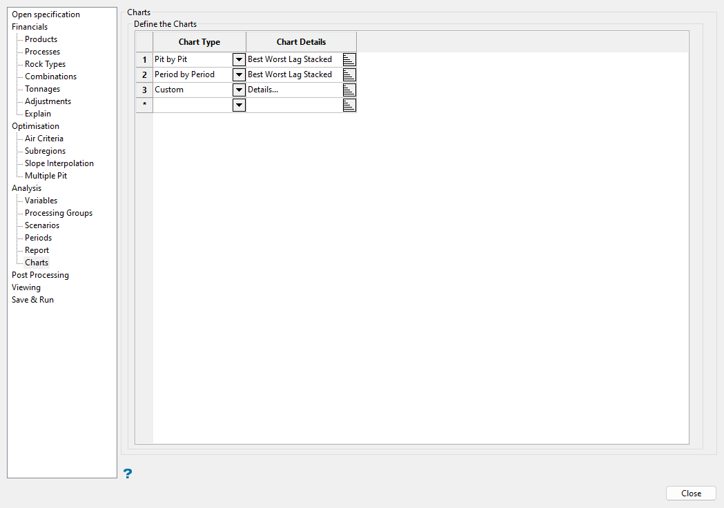
Use this pane to configure the different types of charts to save as tabs in an Excel file.
Note: Select Generate charts on the Analysis pane to activate the Charts options.
Follow these steps:
-
Select the Chart Type from one of the following options in the drop-down list:
-
Pit by Pit: The standard pit by pit chart depicts Total Ore and Waste as stacked columns for each pit plotted against the primary (left) axis. Additionally, a line chart of discounted cash flow plotted on the secondary (right) axis is overlaid for all analysis cases being used (i.e. Best case, Worst case, and/or Bench lag).
-
Period by Period: The standard period by period chart depicts Total Ore and Waste as stacked columns for each period plotted against the primary (left) axis. Additionally, a line chart of discounted cash flow plotted on the secondary (right) axis is overlaid for all analysis cases being used (i.e. Best case, Worst case, and/or Bench lag).
Note: The Period by Period chart type is only available in cases where an analysis scenario is specified.
-
Custom: Use the custom chart to export data not provided by the two standard chart types.
Note: Each row in the Charts grid will generate two new chart tabs in the Excel spreadsheet, named with the chart number followed by the chart type, with one tab displaying the generated visual chart and the other providing the chart data.
-
-
Click
 in the Chart Details field to open the dialog used to define the chart parameters and format.
-
In the Overview tab of the dialog, define preferences for how the information will be presented on the chart.
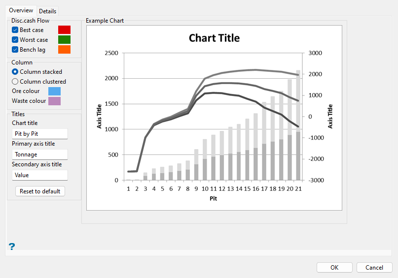
Note: The Overview tab is only available for the two standard chart types.
By default, a line chart of discounted cash flow is overlaid for all analysis cases being used (i.e. Best case, Worst case, and/or Bench lag checkboxes selected in the Disc. cash Flow section). The secondary axis is used for these charts. These line charts can be turned off by deselecting the corresponding checkbox. The colour for these lines may be changed with the colour selection controls to the right of the checkboxes.
Select between the Column Stacked and Column Clustered representation of the Total Ore and Waste variables, and select the Ore colour and Waste colour from the current colour tables. A clustered column chart compares values across categories. A stacked column chart shows the relationship of individual items to the whole, comparing the contribution of each value to a total across categories.
Define the Chart title, Primary axis title (left), and Secondary axis title (right).
At any point, click Reset to default to restore the chart to default values prior to editing. The chart shown on the right of the dialog will only be an example greyscale image, and will not reflect your actual data.
-
In the Details tab of the dialog, assign what data will be shown in the chart and the appearance.
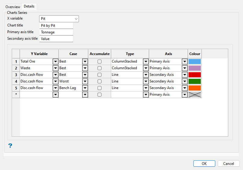
For the standard charts, you can use this tab to customise or add additional datasets. You can also use this tab to define a custom chart.
Note: Customisation of standard charts may result in loss of the chart preview availability in the Overview tab.
Set the X variable for the chart. This field will be populated by default for the standard charts, or you can select a different variable from the drop-down list. The Chart title, Primary axis title (left), and Secondary axis title (right) are pulled from the entries on the Overview tab, if applicable, and you can edit these fields on this tab as desired.
Each row in the grid represents a series in the resulting Excel chart. Select the Y Variable for a series to plot data on the Y axis of the chart from the drop-down list and select the Best, Worst, or Bench Lag analysis type for the data from the Case drop-down list.
Select the Accumulate checkbox if you want to accumulate the value of the variable between successive values of the X variable. When the checkbox is selected, each successive bin of the chart represents a cumulative value of the selected Y Variable.
Example: If Period is the X variable, Rock is the Y variable, and Accumulate is selected, the value of the Rock variable at each successive period will reflect the total for all previous periods.
Next, define how the series will be formatted on the chart. Select the representation (line, column stacked, etc.) of the variable on the chart from the Type drop-down list. Specify on which axis the values will be plotted by selecting Primary Axis or Secondary Axis from the Axis drop-down list. Ensure that quantities in similar ranges and units are plotted on a single axis; that is, product units on one axis and tonnages on another axis. Select the Colour for the series from the current colour table.
Note: Not all chart types are compatible with one another in Excel. See the Microsoft Excel documentation for details.
-
Click OK to save the changes in the dialog and return to the main panel.
-
-
Define more charts as desired in additional rows of the grid by repeating these steps.
Post Processing
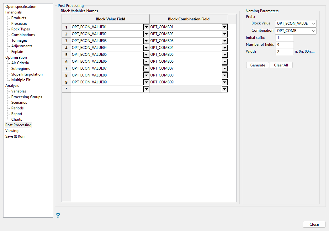
Use this pane to export the economic value and corresponding rock-process combination number computed by the optimiser to block model variable. If multiple pits are generated, each pit uses a different economic value for each block. To account for this, this pane can be used to create a block model variable for each pit.
Follow these steps:
-
Define the block model variable(s) to export the value to in the Block Value Field and Block Combination Field cells. Select an existing variable from the drop-down list, enter a name for a new variable, or follow the next steps to populate these fields using a base prefix name and unique suffixes for multiple pits.
Note: The options for combinations will only be available if Calculate Economic Value is selected in Financials pane.
-
If you are working with multiple pits, use the fields on the right side of the pane to define the prefixes and suffixes to automate creating variable names for the post processing.
-
Select existing block model variables from the Block Value and Combination drop-down lists to define the prefixes, or enter new names for both fields.
-
Enter the Initial suffix to set the value to start with, which will then be used to increment from until the Number of fields value is reached (i.e. maximum suffix value), using the number of digits specified in the Width field.
Example: If Width is set to
2, with an Initial suffix of9, the Number of fields as11, and a Prefix ofPitValue, the variable names generated will bePitValue09,PitValue10, andPitValue11. -
Click Generate to populate the grid with Block Value Field and Block Combination Field entries based on the prefix and suffix entries. You can also click Clear All to clear the grid.
-
Viewing
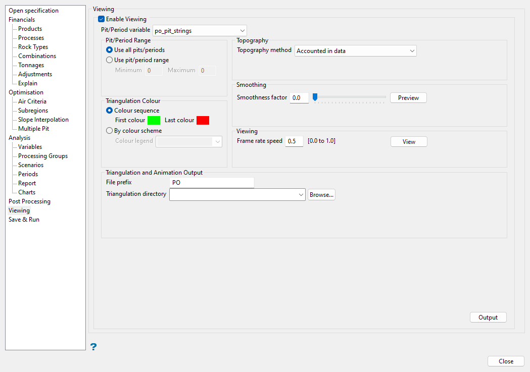
Use this pane to generate triangulation shells and an animation file to visualise the pit, period, or phase output from optimiser.
There are several ways to view pits generated by Pit Optimiser:
-
Block > Pit Optimiser > Viewing... displays pits as triangulations from values stored in a block model variable.
-
Block > Pit Optimiser > Edit – Viewing pane is the same functionality available in Block > Pit Optimiser > Viewing....
-
Block > Viewing > Pits... generates pit strings from a populated block model variable.
Follow these steps:
-
Select the Enable Viewing checkbox to activate the options in the pane, allowing triangulation and animation output.
-
Select the Pit/Period variable of interest from the drop-down list, which contains block model pit, period, and phase variables you have defined in the previous panes.
-
Select whether to Use all pits/periods in the selected variable or Use pit/period range and enter the Minimum and Maximum values of pits/periods to include in the viewing output. A range of 0 represents the unchanged topography.
-
Specify the triangulation colour by selecting either Colour sequence or By colour scheme:
-
Colour sequence: Select this option to colour the output by cycling through the colour palette from the First colour selected to the Last colour selected. If fewer colours are selected than needed, the colours will cycle through the selected range as many times as needed.
-
By colour scheme: Select this option to colour the output based on a predefined Colour legend selected from the drop-down list. The colour legend requires at least as many colours as pit triangulations.
-
-
Select the Topography method from the following options in the drop-down list:
-
Triangulation: Select this option to choose the Triangulation from the drop-down list, or click Browse... to select a file from a different location.
-
Block Model Variable: Select this option to choose the Topography variable from the drop-down list. You must also input the range of values to be considered as air blocks. For the purposes of calculating the topography, any blocks within this inclusive range will be considered as being above the topography.
-
Accounted in data: Select this option if the topography data is accounted for in the Pit/Period variable. The topography may not be accounted for in the block model variable if you did not use the fix for air blocks option in pit optimiser.
-
-
Adjust the Smoothing factor that will be applied to the appearance of the output. A Smoothness factor of
0means no smoothing will be applied, while a value of100will apply the maximum amount of smoothing.Tip: Click Preview to open a window with a real-time preview of the smoothing being applied interactively.
-
Adjust the Frame rate speed to set the speed that the temporary animation will change between triangulations when the animation is played. A Frame rate speed of
1is the fastest speed and0is the slowest.Tip: Click View to create and display a temporary animation of the output triangulations with an animation controls dialog. The View button is intended for temporary viewing purposes; it does not save the output.
-
Configure the Triangulation and Animation Output by entering the File prefix for the names of the triangulations and animation output files and selecting the Triangulation directory for the output triangulations from the drop-down list, which contains all
.trifolders in the current working directory, or enter the name of a new directory with the.triextension. Click Browse... to navigate to a different location.Note: If no Triangulation directory is selected (i.e. the field is left blank), the triangulations will be saved to the current working directory. The animation will always output to the current working directory.
-
Click Output to save the animation file and the triangulations for the shells as specified in the pane.
Save & Run
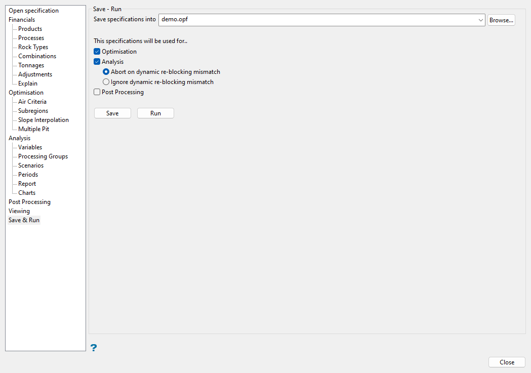
Use this pane to save the parameters to a new or existing specification file (.opf), as well as perform the optimisation, analysis, and/or post processing.
Follow these steps:
-
Specify the specification file (
.opf) to save to or run by entering a new name in the Save specifications into field or by selecting an existing file from the drop-down list, which contains all.opffiles in the current working directory. Click Browse... to navigate to another location.Note: When selecting file names from the drop-down list, the file is not loaded. Instead, whatever values are currently loaded in the panel will overwrite the existing specifications file.
-
Select from the following options to define what the specification will be used for:
-
Optimisation: Select this option to save optimisation parameters or run the pit optimiser. The optimiser will be run before the other options if they are selected.
-
Analysis: Select this option to save analysis parameters or run the analysis tool that generates reports and/or charts. You will need to specify whether to Abort on dynamic re-blocking mismatch or Ignore dynamic re-blocking mismatch. If the Optimisation option is also selected, analysis will run after the optimisation is complete.
Note: The analysis will not run without the optimisation being executed first. The analysis uses the
FPPfile generated in the optimisation to determine which pits and cost factors were used. -
Post Processing: Select this option to save post processing parameters or run the post processing tool. If the other options are selected, post processing will run after the optimisation and analysis are complete.
-
-
Select either Save to save the applicable panel parameters to the specification file (
.opf) or Run to execute the selected options. The Run option also saves the applicable parameters to the specification file.If you choose to run any of the options, a TC Shell window will open and run the process. When the process for one process is completed, press any key to close the TC Shell.
Tip: Use Block > Pit Optimiser > Batch... to run multiple specification files sequentially.

