Method
There are three main methods of creating an Integrated Stratigraphic Model: Stacking, Structural Surfaces, and Hybrid.
Each method has its own advantages and drawbacks. Model Stratigraphy makes it easy to try more than one method, and compare the results. Take careful consideration before choosing the final method.
The following table is provided as a basic guide:
|
Requirement |
Preferred base modelling method |
|---|---|
|
Use of many inclined or curved drillholes |
Structural Surfaces or Hybrid |
|
Use of additional design data on more than one horizon |
Structural Surfaces or Hybrid |
|
Greater control of thickness and burden modelling |
Stacking or Hybrid |
|
Propagation of reference structure through multiple seams |
Stacking or Hybrid |
|
Ensuring no horizons cross |
Any method |
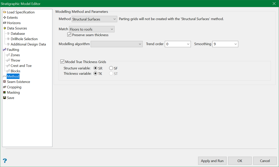
Modelling Method and Parameters
Structural Surfaces Method
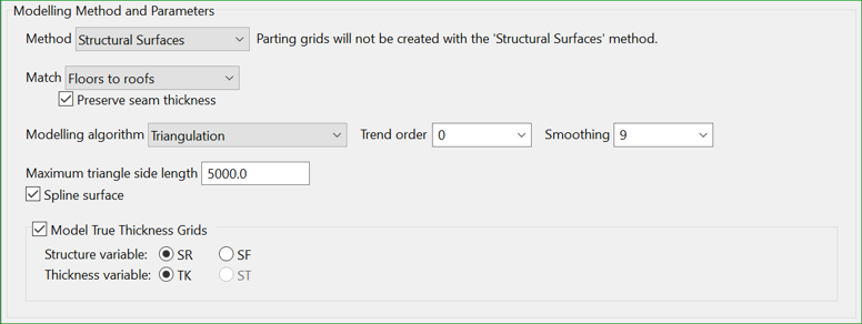
Figure 1 : Structural Surfaces method with a Triangulation modelling algorithm
The Structural Surfaces method models individual roof and floor surfaces for each horizon. As roof and floor surfaces represent the same type of data, a height above sea level, a single modelling method is used for both.
In the example above (Figure 1), a triangulation method is used with a 2nd order trend and 9 Smoothing passes. To avoid very long triangle edges, the Max triangle side length is limited to 5000.
Note: The Max triangle side length field populates to the pane because the Triangulation Modelling algorithm is chosen. Different Modelling algorithm selections will populate the panel with unique fields.
After roof and floor models for each horizon are created, thickness grids are automatically generated between adjacent pairs of surfaces. Every node in each thickness grid is forced to a value of zero or greater, which insures that no horizons cross each other.
Should a horizon cross its neighbour, either the floor is forced to the roof position, or the roof is forced to the floor position. Control the choice made with a selection from the Match drop-down list. (Figure 2)
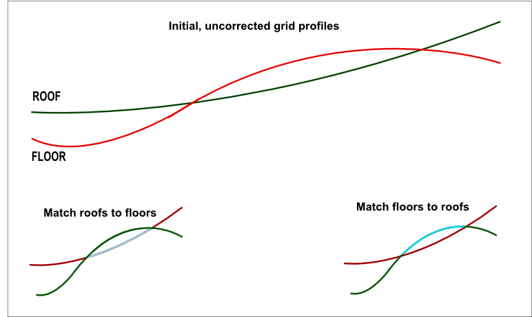
Figure 2 : Result of forcing zero thickness with the Match drop down list.
An iterative process yields good results. Someone with general knowledge of the deposit should review the result of several runs with different Method options to determine the best method. For example, a syncline or anticline would typically respond well to a 2nd order trend.
Tip: Select Geology > Drilling Section tools to view resulting grids in Vulcan.
Stacking Method
Note: If both Fault Blocks and Model throws with dips are enabled, the Stacking method is not available.
The Stacking method creates all horizon models based upon one selected structural surface. The selected surface becomes a reference for creating the rest of the grids in the model. The remaining surfaces are created by adding and subtracting thicknesses and midburdens from the reference surface.
Important The reference surface is the horizon in which there is the most confidence. This is generally the horizon with the most, or most reliable, data.
A check is performed thicknesses prior to addition to ensure that all grid nodes contain a value of zero or greater to avoid horizon crossovers.
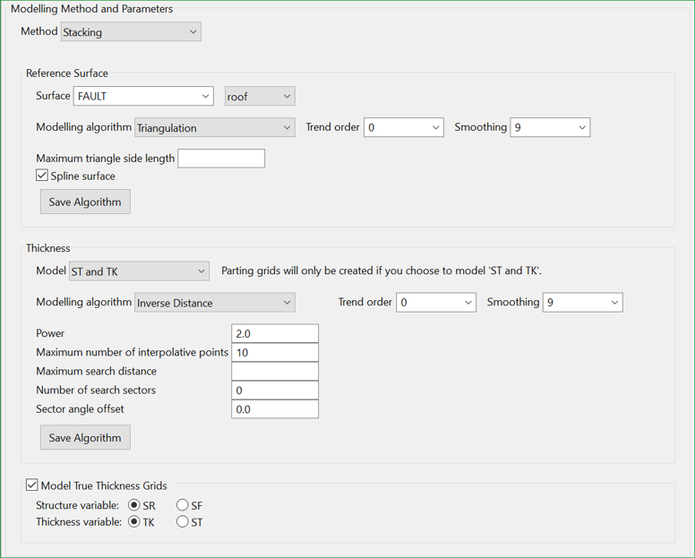
Figure 3 : Example Stacking method configuration
When selecting a Stacking Method, define Modelling algorithms for both the Reference Surface and Thickness grids.
Note: Different Modelling algorithm selections populate the pane with unique fields.
Reference Surface
In Figure 3, the YE horizon is the reference surface. YE is modelled using a Triangulation Modelling algorithm.
Thickness Grids
The Model type can be:
-
ST only
-
ST as TK
-
ST and TK
The abbreviation ST refers to structure thickness. This is the thickness the first logged interval in a horizon to the last logged interval for the same horizon in a single drillhole.
The abbreviation TK refers to product thickness. This is defined as the logged structure thickness minus any logged, in-seam parting thicknesses.
Each thickness (TK or ST) and midburden (MD) grid generates and is checked to ensure that all grid node values are zero are greater before stacked on the reference surface.
It is possible to use a different Modelling algorithm when modelling Thickness grids.
Model True Thickness Grids
Use this option to calculate the true thickness grids. In many cases, the grids only measure the 'vertical thickness' by default, which can overestimate the actual seam thickness for dipping seams. However, the 'true thickness' measures the thickness orthogonal to the dip of the seam and therefore is more accurate.
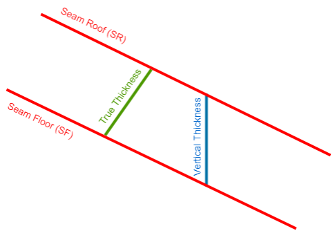
Figure 4 : True Thickness calculation
Hybrid Method
Note: If both Fault Blocks and Model throws with dips are enabled, the Hybrid method is not available.
The Hybrid method is an enhanced Stacking method. The ability to include additional design CAD data for any roof, floor or thickness interval for any horizon adds extra control. Options on the Additional Design Data pane option control the horizontal and vertical influence of defined design data.
A Hybrid method offers many of the advantages of either the Stacking or Structural Surfaces method with few of the drawbacks.
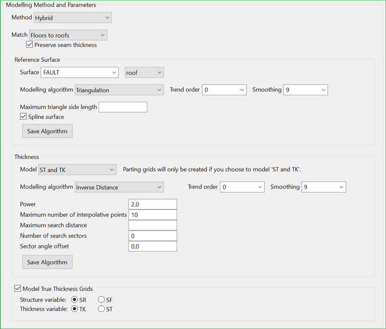
Figure 5 : Example of Hybrid method configuration.
Modelling algorithm
For details on the options available with each modelling algorithm, see Modelling algorithm options. An overview of the algorithms is given below.
- Triangulation: This method is typically used for modelling structural surfaces, such as structure roof and floor and structure thicknesses, and is recommended for modelling deposits with thin bedding planes. The results are a unique interpolated surface that honours all of the raw data values. Using a trend surface with this modelling method allows a regional feature to be applied to the local area of interest.
The triangles are as close to equilateral as possible and have a data point at each vertex. There will be linear interpolation between the three node points that make up each triangle. This method cannot extrapolate values higher or lower than the actual point values, causing the tops of hills and the bottoms of drainage areas to become flat. To avoid this scenario, the triangulation can be manipulated by applying a spline to the surface. The triangle network is covered with a mathematical surface that passes through each data point and is tangential to each point's previously determined slope, resulting in a surface that changes smoothly in all directions. All of the raw data values are honoured and the surface is projected above and below raw data values between data point locations.
This method does not allow for surface extrapolation beyond the raw data point locations. Vulcan uses Trending and Inverse Distance to extrapolate a triangulation to the model's edge.
- Inverse Distance: This method is typically used for modelling thickness and quality information. This method searches concentrically about each grid node for a minimum number of points to use to interpolate the grid node value. The number of points used and the distance to search for these points is specified as part of the method parameters. You can also divide the area into a maximum of 8 sectors, forcing the program to find the closest points in each sector, which is useful if the drillhole data is predominantly found in one section of the modelling area. This method should not be used on faulted datasets or for deposits where the bedding planes are thin.
The grid node values are determined by taking a weighted average of the collected data points. Therefore, the closer a drillhole is to the grid node, the greater the effect it will have on the calculated node value. The weighting used is the inverse of the distance to the nominated power.
- Krige: This method is based on a statistical analysis of spatially located data. The first step in kriging is to perform a variography analysis of the sample data. The resulting variograms express the degree of correlation between samples as a function of distance in several different directions. Sample data are usually correlated at short distances and less correlated at longer distances. Some sample data, such as water table levels, show a high degree of correlation at short distances. Other sample data, such as gold grade, usually show a larger degree of variance even at short distances. All sample data show a correlation approaching zero at larger distances. By fitting a variogram model function to the correlation data we make a function that predicts how well two samples will be correlated given their spatial relationship.
This method estimates a variable at a point by locating and weighting nearby samples. The weights take into account the degree of correlation between each sample and the estimation point, and also the degree of correlation between each pair of samples. The resulting weights provide a de-clustered weighting of the samples that minimises the variance as defined by the variogram.
-
Spline: This method uses a drafter's spline, which is a flexible curve that can be fitted to a sequence of points so that a smooth curve can be drawn between them. The procedure fits a low order polynomial along the grid lines to all adjacent sets of points and from these it interpolates values at the grid points. The spline method demands that the data points lie on the grid lines where the X and Y values are multiples of the grid spacing. Normally, the spline method is used to model string data, such as contours. The tension of the splines may be specified (negative value implies relaxed) as can the bias applied to the splines in the X (vertical bias) and Y (horizontal bias) directions.
-
Least Squares This method is sometimes called a "moving average" because each node in the grid is estimated as the average of values from control points in a neighbourhood that is moved from grid node to grid node. First, all control points are located that reside in a specified neighbourhood around the grid node to be estimated. The values of these points approximately define a sloping plane or low order polynomial. Secondly, the equation of the plane is calculated and used to estimate the value of the grid node. The process of fitting a plane and evaluating it to estimate the surface is repeated for every node on the grid.
-
Trend Surface: This method is based on the premise that small-scale features are masked and distorted in maps that are dominated by large scale, high amplitude features. Consequently, if the large-scale features are removed, then the smaller features are more easily identified and evaluated. This method applies a specified regional trend to the modelling process and then allows you to evaluate the residuals, or differences between the raw data values and the regional geological trend of the area.
First, a smooth regional map called a "trend surface" is made, this is a two dimensional global polynomial function. Then the differences between the original data point values and the smooth regional trend are calculated to produce a "residual" map (which displays the local features). Both maps may be significant in the geological interpretation.
Polynomials of degree 1, 2 and 3 are known as linear, quadratic, and cubic polynomials. A polynomial of degree 1 is a straight line if it is two dimensional or a plane if it is three dimensional. Every polynomial of degree 2 is a parabola with a vertical axis of symmetry that represents an anticlinal or synclinal shape. A third order polynomial defines an undulating surface. The third order trend may be applied to regional areas where both an anticline and an adjacent syncline are present or regions where the strata is actually folded. Higher order polynomials are not representative of geological surfaces. They tend to oscillate wildly between the outside control points and may generate very distorted values near the model's edge. How well the surface statistically fits the data can be determined from the "Goodness-of-fit" information produced during the modelling process.
-
Radial Basis Function (RBF): The Radial Basis Function (RBF) is a system of linear equations that are solved to derive weights and drift model coefficients for each sample. Due to the non-intersecting behaviour of this option, it effectively allows veins and coal seams to be modelled. The input data for the modelling process could be CAD data (points, lines, polygons), ribbons, drill holes, and triangulations. For a surface created from CAD data, such as lines and polygons, the constituent points will be sitting on the surface. For drilling data or attributed data, it creates a surface interpolated from points matching defined values. RBF only models a single unit at a time and can produce surfaces, a single closed solid, or points of the surfaces.
Trend Order
Specify the triangulation trend order. Refer to the Trend option (in Grid Calc > Data ) for more information.
Smoothing
Specify the number of smoothing passes to be applied to the grid once it has been created. Smoothing applies a mathematical equation that calculates the variance of the modelled data. Once the value has not changed from the previously calculated variance by a certain percentage, the iterations or calculation process are discontinued. Usually nine smoothing passes are sufficient.
Modelling algorithm options
Triangulation
Max triangle side length
Enter the maximum triangle side length. Any grid node that falls in a triangle with a side length that exceeds this value is masked. The default is 'unlimited'.
Note: The default mask - the one that results from the data distribution and modelling technique - may (and can) be altered or replaced by subsequent masking processes, for example, crop lines.
Spline surface
Enter a value for the spline tension. A negative value relaxes the splines, therefore the higher the negative value the more relaxed the splines will be, that is, they curve more. A positive value increases the spline tension, it makes the splines pull tight over the control points, reducing, for example, the height of the tops of hills and the depth of valleys. The values are usually in the range of -3 to 3, but they can be more or less.
Inverse Distance
Power
Enter the power to be used when calculating the weighting for the data points.
Max num interpolative points
Enter the number of data points to use when interpolating values.
Specify the number of interpolative points to be used by the inverse distance method (the default value is "10").
Max search distance
Enter the maximum distance in which to search for interpolative points. Nodes that require points further than this distance are masked. However, they do have interpolated values derived using all the required points regardless of the distances, and such nodes may easily become 'visible' should the default mask be altered.
Specify the maximum search radius for the inverse distance method. Grid points evaluated using points further than this distance from the grid point will have a data mask value of zero. The default is unlimited search distance.
Num search sectors
Enter the number of search sectors (a maximum of "8"). This option to divide the search area into sectors so that data selected for modelling does not come from a cluster of points. Usually 8 sectors are used.
Sector angle offset
Enter an angle, in degrees, for the offset of the sectors. For example, if you choose to have 6 sectors and a sector angle offset of 0°, then the first sector extends from a bearing of 0° to a bearing of 360 · 6 (360 divided by 6)=60°. However, if the number of sectors is 6 and the sector angle offset is 5°, then the first sector extends from a bearing of 5° to a bearing of 60+5=65°. Rotating the sectors can stop samples being located on a boundary, which can cause problems as there is no way to determine into which sector a sample is placed if it is on a border.
Krige
Max triangle side length
Enter the maximum triangle side length. Any grid node that falls in a triangle with a side length that exceeds this value is masked. The default is 'unlimited'.
Note: The default mask - the one that results from the data distribution and modelling technique - may (and can) be altered or replaced by subsequent masking processes, for example, crop lines.
Max num interpolative points
Enter the number of data points to use when interpolating values.
Note: If, in the data set being modelled, there are fewer points available than the number of interpolative points specified, then the number of available points will be used as the specified number of interpolative points. This means that a model will always be produced.
Max search distance
Enter the maximum distance in which to search for interpolative points. Nodes that require points further than this distance are masked. However, they do have interpolated values derived using all the required points regardless of the distances, and such nodes may easily become 'visible' should the default mask be altered.
Num search sectors
Enter the number of search sectors (a maximum of "8"). This option to divide the search area into sectors so that data selected for modelling does not come from a cluster of points. Usually 8 sectors are used.
Sector angle offset
Enter an angle, in degrees, for the offset of the sectors. For example, if you choose to have 6 sectors and a sector angle offset of 0°, then the first sector extends from a bearing of 0° to a bearing of 360· 6 (360 divided by 6)=60°. However, if the number of sectors is 6 and the sector angle offset is 5°, then the first sector extends from a bearing of 5° to a bearing of 60+5=65°. Rotating the sectors can stop samples being located on a boundary, which can cause problems as there is no way to determine into which sector a sample is placed if it is on a border.
Model name
Select Spherical, Exponential or Gaussian as the variogram model type.
Nugget of variogram
Enter the standardised nugget value returned from variogram analysis. The value returned (between 0 and 1) is the proportion of the variogram model sill represented by the variogram model nugget.
For example, if the variogram model nugget value is '0.4', and the variogram model sill value is '2.0', then the nugget entered will be 0.4· 2.0 = 0.2.
Note: The sill value does not need to be entered as its standardised value will be set as '1'.
The following fields define the shape and size of the variogram.
Bearing to major direction
Enter the bearing of the major axis of the ellipse.
Major range to the sill
Enter the length of the major axis. This is the distance from the centre of the ellipse to its edge in the major direction.
Minor range to the sill
Enter the length of the minor axis. This is the distance from the centre of the ellipse to its edge along the minor axis. The minor axis is perpendicular to the major axis.
For example, if bearing = 90, major = 25 and minor = 15, then the ellipsoid is 50 long in the East/West direction, 30 wide in the North/South direction, and the major axis is parallel to the East/West axis.
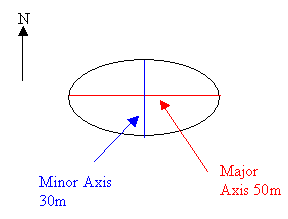
Figure 6 : Example ellipse
If the bearing = 0, major = 25 and minor = 15, then the ellipsoid is 50 long in the North/South direction, 30 wide in the East/West direction, and the major axis is parallel to the north-south direction.
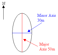
Figure 7 : Example ellipse
Click OK.
The points will be modelled.
Spline
The Spline method cannot work with mapfile data.
Max triangle side length
Enter the maximum triangle side length. Any grid node that falls in a triangle with a side length that exceeds this value is masked. The default is 'unlimited'.
Note: The default mask - the one that results from the data distribution and modelling technique - may (and can) be altered or replaced by subsequent masking processes, for example, crop lines.
Spline surface
Enter a value for the spline tension. A negative value relaxes the splines, therefore the higher the negative value the more relaxed the splines will be, that is, they curve more. A positive value increases the spline tension, it makes the splines pull tight over the control points, reducing, for example, the height of the tops of hills and the depth of valleys. The values are usually in the range of -3 to 3, but they can be more or less.
Least Squares
The Least Squares method is not a data honouring method.
Max triangle side length
Enter the maximum triangle side length. Any grid node that falls in a triangle with a side length that exceeds this value is masked. The default is 'unlimited'.
Note: The default mask - the one that results from the data distribution and modelling technique - may (and can) be altered or replaced by subsequent masking processes, for example, crop lines.
Spline surface
Enter a value for the spline tension. A negative value relaxes the splines, therefore the higher the negative value the more relaxed the splines will be, that is, they curve more. A positive value increases the spline tension, it makes the splines pull tight over the control points, reducing, for example, the height of the tops of hills and the depth of valleys. The values are usually in the range of -3 to 3, but they can be more or less.
Trend Surface
Max triangle side length
Enter the maximum triangle side length. Any grid node that falls in a triangle with a side length that exceeds this value is masked. The default is 'unlimited'.
Note: The default mask - the one that results from the data distribution and modelling technique - may (and can) be altered or replaced by subsequent masking processes, for example, crop lines.
Spline surface
Enter a value for the spline tension. A negative value relaxes the splines, therefore the higher the negative value the more relaxed the splines will be, that is, they curve more. A positive value increases the spline tension, it makes the splines pull tight over the control points, reducing, for example, the height of the tops of hills and the depth of valleys. The values are usually in the range of -3 to 3, but they can be more or less.
Related topics
-
Data Source(s)
-
Faulting

