Zone-based graphs
Source file: zone-based-graphs.htm
Zone-based graphs plot variables derived by averaging cell-based values over all the cells in a single zone. A zone-based graph can display data for multiple zones at once; each zone is plotted with its associated colour. All zone-based graphs derive from data acquired from the scanner.
The most important zone-based graphs in Sentry are based on cell displacement, which in turn is based on cell range:
-
Cell range is the average distance from the scene origin to the scan points contained in a cell.
-
Cell displacement for a cell in a given scan is defined as the difference in range between the cell in the measurement base and the same cell in the scan. Positive displacement values indicate movement towards the scanner, while negative displacement values indicate movements away from the scanner.
There are four zone-based graph types, all of which are derived from scanner data:
|
|
Displays trends of average cell displacement over all cells within each selected zone. |
|
|
Displays trends of average cell displacement per unit time over all cells within each selected zone. |
|
|
Displays the inverse of velocities as data points. Also displays a line of best fit for points immediately before to the time slider to project likely time to failure. See Line fitting window Note: Inverse velocity graphs can be based on either raw or smoothed velocities, as configured in Preferences. See Preferences > Graph . |
|
|
Displays the average laser intensity over all cells within each selected zone, for each scan. |
|
|
|
Zone based graph options |
Smoothing
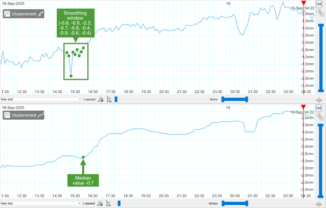
All zone-based graphs (with the exception of inverse velocity with line fitting) can have smoothing applied to them to reduce the amount of noise and reveal general trends within the data. The smoothed value for any point in time is defined as the median of the values within the smoothing window up to that time.
Note: The larger the smoothing window is, the longer it will take for real changes in the underlying data to appear.
|
|
|
Determination of smoothed value. Unsmoothed displacement graph (top) and smoothed (bottom). |
-
To smooth all zone-based graphs automatically,
 Default Smoothing Window.
Note: The Default Smoothing Window field includes buttons that increment or decrement the fitting window in 30 minute steps. This is useful for making quick comparisons between smoothing windows.
-
To apply smoothing to the current graph temporarily, drag the dynamic smoothing window slider, found below the graph view. Dynamic smoothing is only applied while dragging the slider control; after releasing the mouse button, the smoothing window will revert to its default.
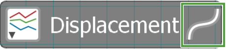
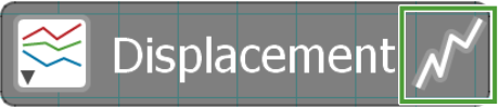
The graph type icon indicates whether smoothing is applied to the graph or not.
|
|
|
|
Graph type indicator with smoothing (left) and without (right) |
|
Velocity window
Velocity-based graphs (i.e. velocity and inverse velocity) plot their data using an average velocity function, defined as the change in displacement over some time period. In Sentry, this time period is called the velocity window. The velocity window can be set to any whole number of minutes greater than 0. However, there is no value in setting the velocity window smaller than the actual scan time. The velocity at any given time is the displacement divided by the velocity window.
The start of the velocity window is unlikely to coincide with an earlier scan. Therefore, the displacement at the beginning of the window is interpolated from the neighbouring data points.
The following image shows the velocity graph using a 300 minute velocity window and the corresponding distance graph used to calculate the velocity.
|
|
|
Velocity window on displacement graph (top) and corresponding velocity calculation (bottom). |
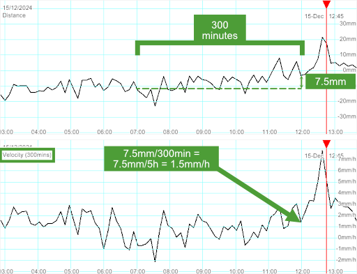
Each point in the velocity graph is determined by the difference in range between its corresponding point in the distance graph and a point 300 minutes earlier in the displacement graph.
With larger velocity windows there will be more lag in the calculated velocities. The velocity graph will also be less variable, with the amount of local noise being reduced.
Note: Significant differences in scans may occur between day and night, depending on diurnal weather patterns. If this is a concern, we suggest a default velocity window of 1,440 minutes (one day).
The velocity window is independent of the smoothing window (discussed above), although both have the effect of smoothing the graph. Smoothing is applied to displacements first; velocity is calculated from the smoothed displacements.
-
To set the velocity window directly, on the Home tab, in the Graph group, enter the period in the Velocity Window field.
Note: The Velocity Window field includes buttons that increment or decrement the fitting window in 30 minute steps. This is useful for making quick comparisons between velocity windows.
Line fitting window
Inverse velocity graphs have a Line fitting window input field instead of a smoothing window slider. The value entered is the period immediately before the time slider over which the line of best fit is determined. The line fitting window is indicated by a blue-shaded area to the left of the time slider.
|
|
|
Determining inverse velocity |
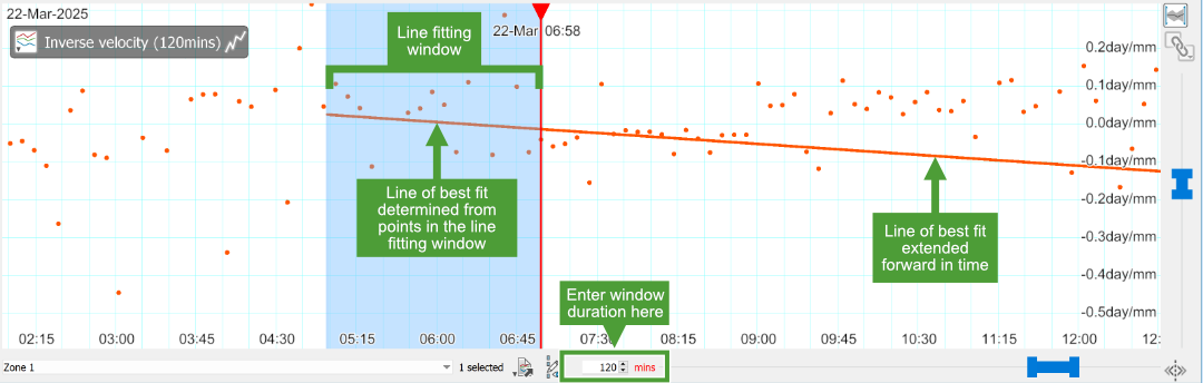
Note: The line fitting window field includes buttons that increment or decrement the fitting window in 30 minute steps. This is useful for making quick comparisons between line fitting periods.
Filtered data
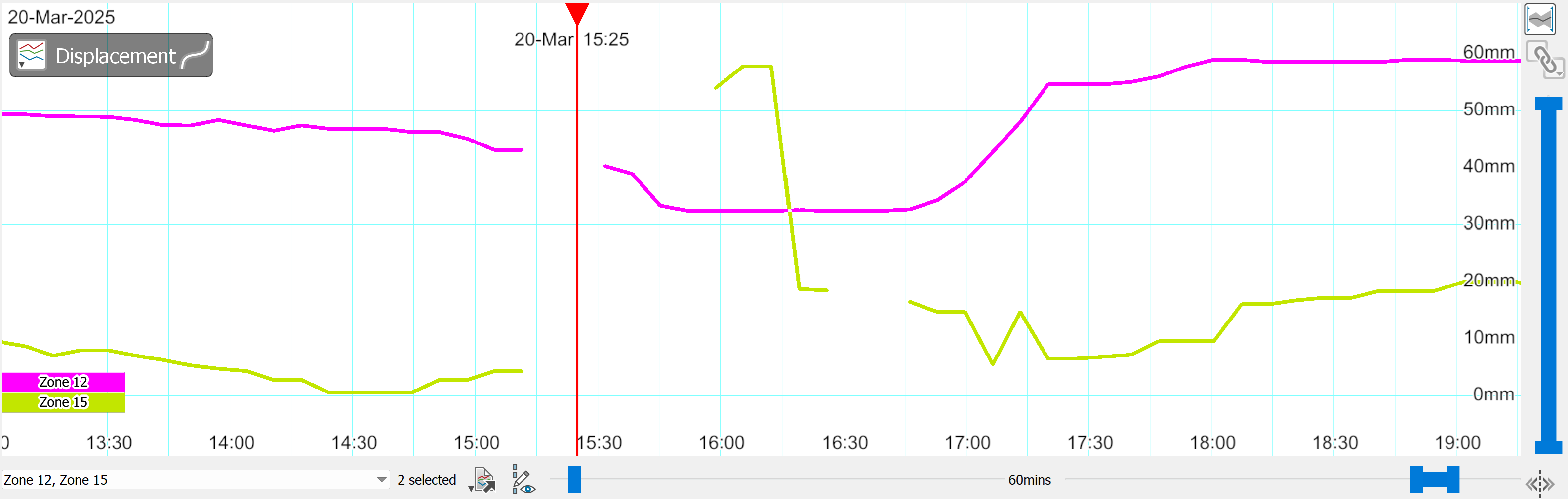
When a zone has no cell data or doesn't meet the chosen Minimum zone cell coverage (see Filtering), there will be a corresponding gap in that zone’s graphs.
|
|
|
Displacement graphs with gaps |
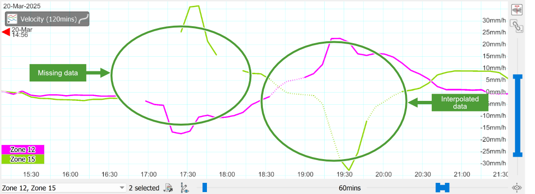
Where this occurs, the velocity graph will have a second gap that is one velocity window further along because the initial displacement for the velocity calculation is missing. The second gap is bridged with a dotted line to indicate that the starting displacement has been interpolated from the scans at either end of the first gap.
|
|
|
Velocity graphs with gaps and interpolated lines |
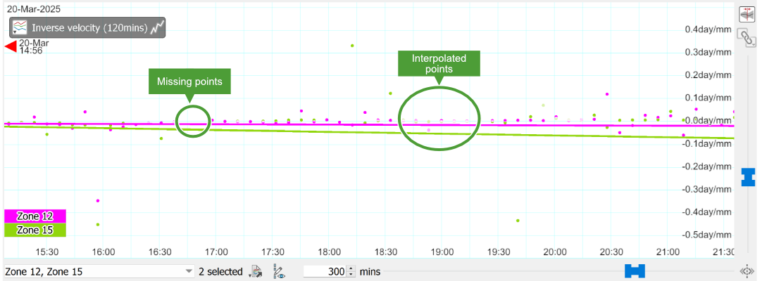
In the inverse velocity graph, the first gap will have no points and the points in the second gap will be faded.
|
|
|
Inverse velocity graphs with gaps and faded points |
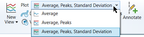
Plot styles
Displacement and intensity graphs can display optional extra information in addition to the average plot. The three possible plot styles are:
To set the plot style, on the Home ribbon tab, in the Graph group, select an option from the Plot list.
|
|
|
Displacement graph showing plot styles |
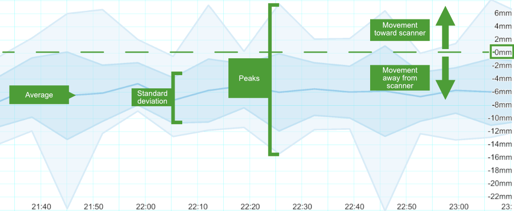
The Peaks and Standard Deviation plots are only shown when the following conditions are met:
-
Only one zone is selected.
-
No smoothing is applied (smoothing window is 0 minutes).
-
The graph type selected is either Displacement or Intensity.
