Timing
Source file: timing.htm
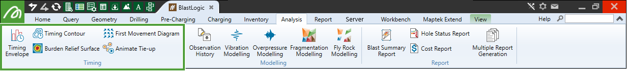
The Timing group of the Analysis tab contains tools that calculate and display different detonation timing properties of a tie-up.
Timing Envelope
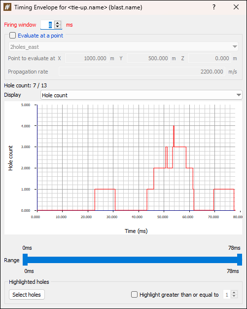
The ![]() Timing Envelope displays a graph depicting the following detonation properties over time (ms):
Timing Envelope displays a graph depicting the following detonation properties over time (ms):
- Detonation count
- Hole count
- Detonation mass (kg)
- Detonation energy (MJ)
- Peak particle velocity (mm/s)
- Max pressure (dB)
These values are determined over a user-specified timing window (usually 8 ms).
To enter the ![]() Timing Envelope tool, follow these steps:
Timing Envelope tool, follow these steps:
-
Place the required tie-up in the view window.
Go to the Analysis tab > Timing group and select
 Timing Envelope.
Note: You can also access this tool from the tie-up context menu. To do so, right-click on the tie-up in the

Tie-upscontainer and select Model > Timing Envelope....The Timing Envelope panel will appear.
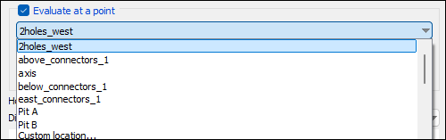
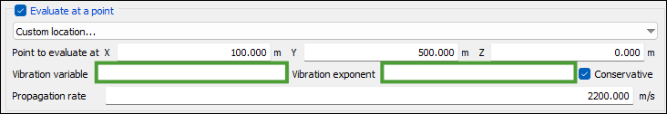
You can calculate and evaluate the timing envelope from the blast to the specified point with the specified propagation rate by selecting the Evaluate at a point checkbox. This is either calculated at a site location that you select from the drop-downor at a custom point when you select Custom location... from the drop-down.
Note: When you select Custom location... from the drop-down, you must also specify the X, Y, Z coordinate, and the Propagation rate field. 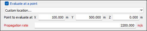
If you leave the Evaluate at a point option unchecked, the ![]() Timing Envelope tool will evaluate the timing envelope at the blast (assuming there is no propagation rate).
Timing Envelope tool will evaluate the timing envelope at the blast (assuming there is no propagation rate).
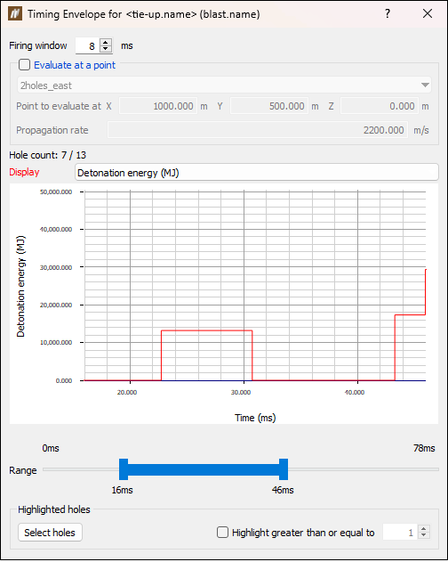
You can zoom the graph by adjusting the Range slider at the bottom of the panel. The values displayed above the slider are the minimum and maximum values that can be set for that range, whereas the values displayed below the slider show the currently set range. Using the Display drop-down, you can set the Y axis to display Hole count, Detonation count, Detonation mass (kg), Detonation energy (MJ), Peak particle velocity (mm/s), or Max pressure (dB).
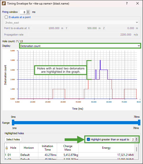
To highlight specific groups of holes in the view window, select the Highlight greater than or equal to checkbox and enter the required value. This is useful for easily locating holes and adjusting the tie-up around them to correct the timing envelope.
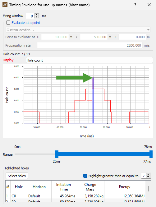
In your view, you can also highlight individual peaks on the graph by double-clicking on them. This can help you determine which holes correspond to the specific peaks of the maximum instantaneous charge when there are multiple peaks with the same charge mass.
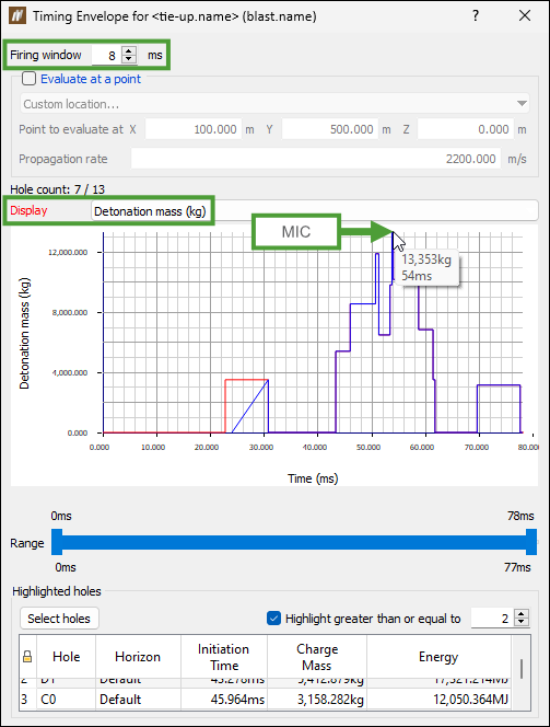
Estimating maximum instantaneous charge (MIC)
Follow these steps to use the timing envelope histogram to estimate MIC for a specified firing window:
-
Specify the required Firing window in the Timing Envelope panel.
Note: Typically 8 ms is used to estimate MIC for non-electronic tie-ups, and 1 or 2 ms is used for electronic tie-ups.
-
Select Detonation mass from the Display drop-down.
-
Hover the mouse over the highest column in the histogram to display the mass value (the MIC for the blast).
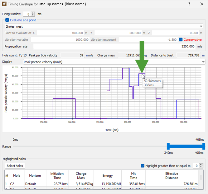
Peak particle velocity
Follow these steps to have BlastLogic calculate a particle velocity graph for a specified firing window:
-
Specify the required Firing window.
-
Select the Evaluate at a point checkbox and choose a location close to the blast(s).
-
Select Peak particle velocity from the Display drop-down.
Note
When calculating PPV, you can choose to apply a conservative or non-conservative approach.
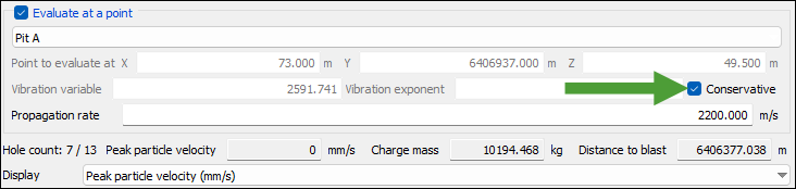
The conservative approach takes into account the closest distance from the point of detonation to the point of observation, which helps to model the worst case scenario. On the other hand, the non-conservative approach calculates the weighted average using the mass of explosives, which is a more technically sound method for modelling the resulting particle velocity. Consequently, the conservative approach can be regarded as
 ,
,
whereas the non-conservative approach, where multiple detonations are taken into consideration, can be calculated for all contributing detonations according to the formula ,
,
where is the distance to each detonation, and
  is the associated charge mass.
Based on these calculations, the resultant modelled particle velocity is calculated according to the formula
 ,
,
where is the site variable,
  is the effective distance,
  is the total charge mass, and
  is the site exponent.
This is calculated for every timing window to determine the subsequent particle velocity for that time period. The maximum calculated particle velocity over the entire blast is reported as the predicted PPV for that receiving position. -
For custom locations or locations with no default values, enter the Vibration variable and Vibration exponent.
-
Based on the data that you provide, BlastLogic Help will display the following information:
-
The peak particle velocity reached by the whole blast.
-
The charge mass, which is the cumulative total of all the detonations contributing to the peak particle velocity.
-
The distance between the blast and the detonation that contributed to the peak particle velocity.
Note: The distance to detonation is calculated using either the conservative or non-conservative approach, as detailed above.
Note
The same values will be generated when you inspect your data using the
 Vibration Modelling tool (see Vibration Modelling for more information).
Timing Envelope panel 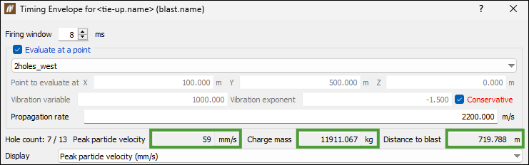
Vibration Modelling panel 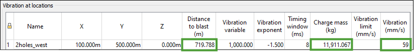
Tip: Hover the mouse over the required column in the histogram to view the peak particle velocity at different time intervals. The peak particle velocity will be displayed both in mm/s and ms units.
-
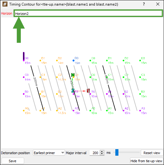
Timing Contour
Use timing contours to visualise the timing between nearby holes to identify patterns and infer the direction of rock movement.
Follow these steps to create a timing contour:
-
Place the required tie-up into the view window.
-
Go to the Analysis tab > Timing group and select
 Timing Contour.
Note: You can also access this tool from the context menu of the tie-up design. To do so, right-click on the tie-up in the
Tie-upscontainer and select Model > Timing Contour.... -
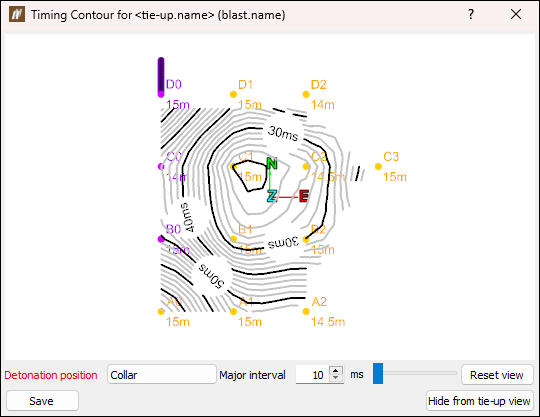
Adjust your view by selecting Collar, Earliest primer, or Toe from the Detonation position drop-down. You can set the interval for the major contours by entering the new value in the Major Interval field or using the range slider.
-
For an electronic tie-up with multiple timing horizons, choose the horizon to view by selecting the required option from the drop-down.
Note: Each timing horizon has different initiation times.
See also: Create Tie-up Design
Note: A pyrotechnic tie-up will show the surface initiation timing curves.
-
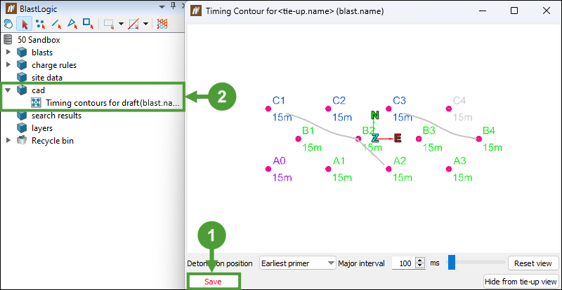
Press Save to create a new object in the cad container. The object will contain the lines and labels that make up the timing contour.
-
Press Hide/Show from tie-up view to remove or add the timing contour from the view that contains the tie-up that the timing contour is based on.
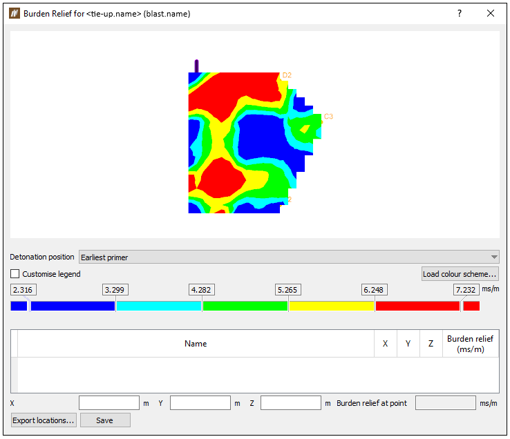
Burden Relief Surface
Burden relief is the amount of detonation time delay per metre of burden at a given location. It is calculated by dividing the time taken to detonate a hole by the hole's distance (in metres) from the free face, which is the area where material is transferred to upon explosion.
To create a burden relief surface, follow these steps:
-
Place the required tie-up design into the view window.
-
Go to Analysis tab > Timing group and select
 Burden Relief Surface.
Note: You can also access this tool from the context menu of the tie-up design. To enter it, right-click on the tie-up in the
Tie-upscontainer and select Model > Burden Relief Surface... . -
For an electronic tie-up with multiple timing horizons, choose the Horizon to view. Each timing horizon has a different burden relief surface.
Note: The surface is displayed alongside the blast with colours according to the legend.
You can evaluate the burden relief at a point by first clicking in the X field, and then clicking on a point in the surface. -
Specify the detonation position by selecting Collar, Earliest primer, or Toe from the drop-down.
-
Specify the required colour scheme as follows:
-
To load a previously created custom colour scheme, click the Load colour scheme... button. This will allow you to load a colour scheme that you have saved in the Custom colour schemes panel (Home tab > Setup group >
 Site).
Important: Only colour schemes that have their Dimension specified as Inverse velocity can be loaded. See Load for more information.
-
To edit the colour scheme, click the Customise legend checkbox . You will be able to edit intervals and colours.
Note: To save the colour scheme, right-click on the set colour scheme and select Copy, then create a new colour scheme in the Custom Colour Schemes panel (Home tab > Setup group>
Site) by specifying its name and pasting the copied colour scheme by right-clicking on the colour bar below the table.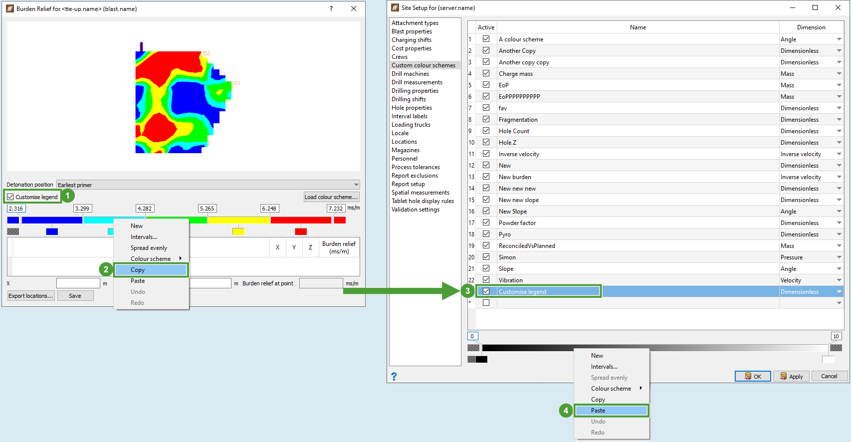
See Custom colour schemes for more information.
-
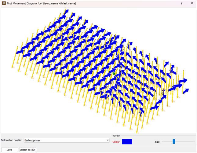
First Movement Diagram
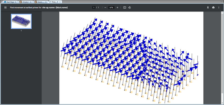
The ![]() First Movement Diagram tool displays the direction that the rock is expected to move after detonation at each point.
First Movement Diagram tool displays the direction that the rock is expected to move after detonation at each point.
To use this tool, follow these steps:
-
Place the required tie-up design into the view window.
-
Go to Analysis tab > Timing group and select
 First Movement Diagram.
 Note: You can also access this tool from the context menu of the tie-up design. To enter it, right-click on the tie-up in the
Tie-upscontainer and select Model > First Movement Diagram.... The First Movement Diagram panel will appear.
-
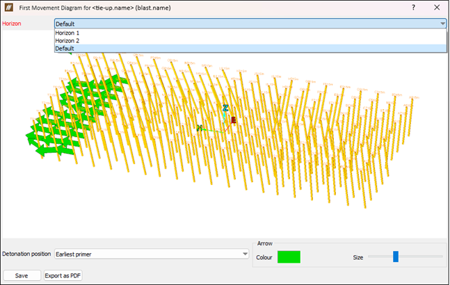
For an electronic tie-up with multiple timing horizons, choose the Horizon to view by selecting the required option from the drop-down. Each timing horizon will have different firing times.
-
Specify the Detonation position by selecting Collar, Earliest primer, or Toe from the drop-down.
Collar 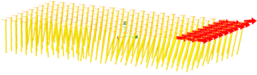
Earliest primer 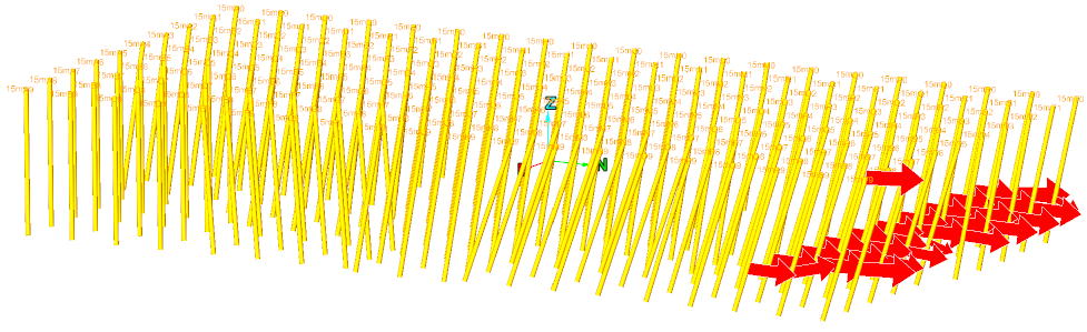
Toe 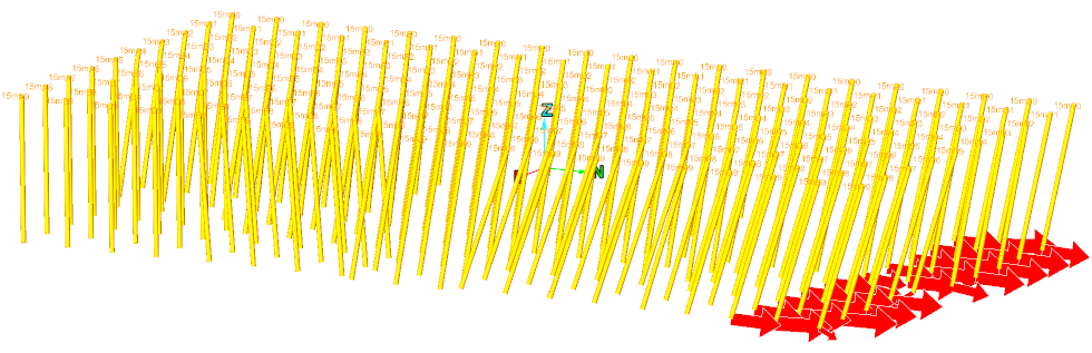
-
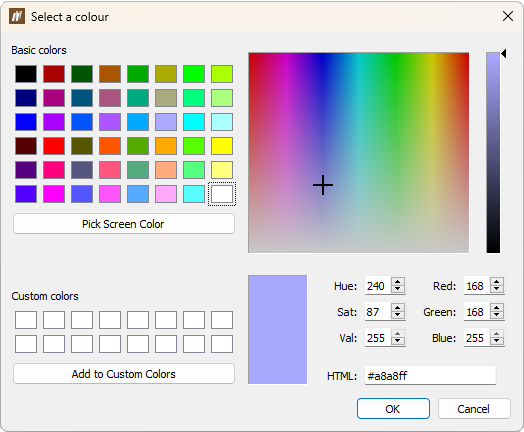
To change the colour of the arrows in your view, click the Colour box field and select the colour from the colour grid.
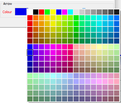 Tip
TipDouble-click the Colour box field to open Select a colour window with detailed colour settings.
-
Move the slider next to the Size heading to adjust the size of arrows in your view.
-
Select Save to save the applied changes. The first movement diagram will be saved in the

site datacontainer in project explorer.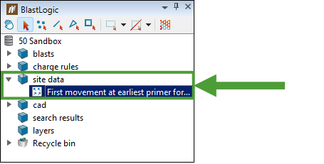
-
Select Export as PDF to generate a ready to save and print First Movement Diagram file.
Animate Tie-up
The ![]() Animate Tie-up tool visualises the detonation sequence of the selected tie-up design.
Animate Tie-up tool visualises the detonation sequence of the selected tie-up design.
To use the tool, follow these steps:
-
Place the required tie-up design into the view window.
-
Go to Analysis tab > Timing group and select
 Animate Tie-up.
 Note: You can also access this tool from the context menu of the tie-up design. To enter it, right-click on the tie-up in the
Tie-upscontainer and select Model > Animate Tie-up....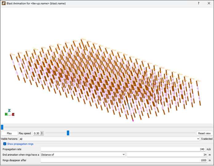
-
Customise your tie-up animation by setting the Play speed and Visible horizons fields.
-
Optionally, select the Show propagation rings checkbox to display the propagation rings that visualise the detonation shock wave through the blast. Next, set the following fields:
-
Propagation rate, by entering the value in m/s unit.
-
End animation when rings have a, by setting an appropriate value and selecting one of the options from the drop-down menu:
-
Time after last detonation of
-
Time after initiation of
-
Distance of
-
-
Rings disappear after, by entering the distance.
-
-
Play or pause the animation with the Play/Pause button. You can use the slider to manually view individual frames of the animation.
Animation when Show propagation rings checkbox
is unselectedAnimation when Show propagation rings checkbox
is selected
