Creating a Cross Orthogonal Variogram
Use this option to calculate a Cross Orthogonal Variogram based on two variables, allowing you to adjust the orthogonal variogram for the two variables and the cross variogram between them, making it easier to handle LMC Validation.
See also: Tutorial - Chart Viewing and Exporting
On the Variography tab, in the Charts group, click Cross Orthogonal Variogram.
When you click Cross Orthogonal Variogram in the ribbon, the Properties panel on the right will populate with various options.
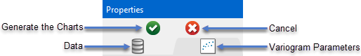
Generate the Charts
Click the green check ![]() icon at the top of the Properties column to generate the variogram charts. You can set the parameters for your variograms before or after creating the initial variograms.
icon at the top of the Properties column to generate the variogram charts. You can set the parameters for your variograms before or after creating the initial variograms.
Cancel
Click the red X  icon to cancel generating the chart. Note that clicking Cancel will also deselect any variables you have selected.
Variogram Parameters tab
Axis Settings
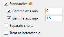
Standardise Sill
Select this checkbox if you want to standardise the variogram sill by dividing the results by the sample variance. This is useful when calculating a semivariogram because instead of reaching the sill at the sample variance it will reach it at 1.
Gamma axis min / max (Optional)
Select one or both of these options if you want to set the minimum or maximum extents of the gamma axis.
Separate Charts
Select this option to display separate charts for each set of variogram parameters.
Treat as heterotopic
Treat selection for each variable as different with respect to the other. Since a cross variogram measures the difference between two variables at a given location, a problem arises when the locations of sample points between the two datasets are different. Select this option to perform heterotopic cokriging when you are working with unequally sampled data and multiple databases.
Direction Settings - Plane
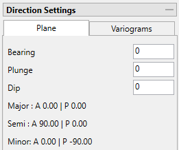
Enter the Bearing, Plunge, and Dip.
Note: The Major, Semi-major, and Minor azimuth and plunge directions are displayed, but cannot be edited from this tab. To edit these settings, click the Variograms tab. Any edits made there will be reflected on this tab.
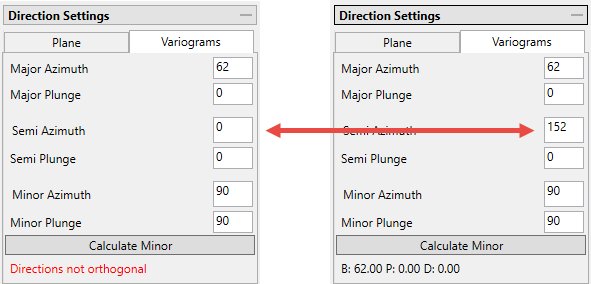
Direction Settings - Variograms
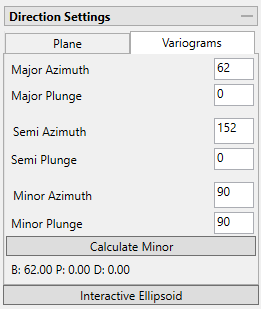
Enter the Major, Semi-major, and Minor Azimuth and Plunge.
Click the Calculate Minor button to automatically fill in the values for the Minor direction.
If entries are made that do not reflect proper orthogonal angles, then the box will be highlighted in red.
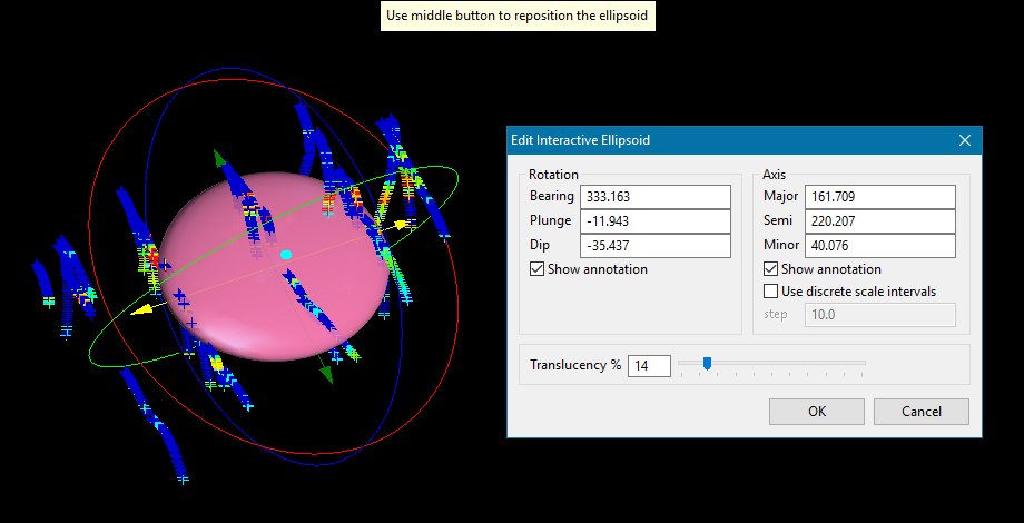
Click the Interactive Ellipsoid button to open an interactive window in the Vulcan 3D viewer. You can use the controls on the ellipsoid to set the direction parameters.
Data Analyser allows you to input the plane orientation and from there obtain the three variogram directions. This can be done before or after the chart has been created. The input plane is the same used in the model for that variable.
The angles for Major, Semi-major, and Minor are automatically calculated from the settings entered in the Plane tab, however, you can edit those settings if you desire. If the Semi-major is not orthogonal (90 degrees) to the Major, then a warning will be given. However, it is not required that the angles be orthogonal to each other. If you want the minor angle to be orthogonal to the Major and Semi-major, then click the Calculate Minor button and the two angles will be automatically filled in.
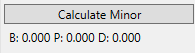
Click the Calculate Minor button to perform the calculation. The results will provide the bearing, plunge and dip based on the Major Azimuth.
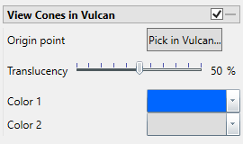
View Cones in Vulcan
You can visualise the search ellipses by enabling the option to View Cones in Vulcan, or by clicking Display Cones from the Connectivity tab in the ribbon. The cones are interactive, therefore, any changes made in the variogram parameters will be automatically reflected in the cones seen in Vulcan.
Steps
-
Begin by clicking the button labelled Pick in Vulcan.
-
In the Envisage workspace, click where you want the origin of the cones to be displayed.
-
Use the slider to adjust the Translucency of the cones.
-
Set the colours for the cone by clicking on Colour 1 and Colour 2, then selecting a colour from the palette.
-
To remove a the cone from the screen, disable the View Cones in Vulcan checkbox.
After you have set the parameters for a cone, it can be displayed using the buttons found on the Connectivity tab on the ribbon.
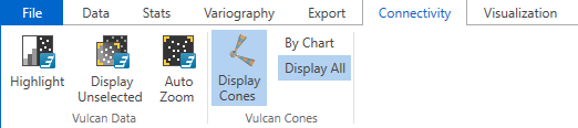
Click Display Cones, then select either By Chart or Display All.
By Chart - Only the charts that have the View Cones in Vulcan option enabled will be displayed.
Display All - All cones will be displayed regardless of whether or not the View Cones in Vulcan option has been enabled.
Primary Major, Semi-major and minor Parameters
Note: The input tabs for all the directions are set up the same.
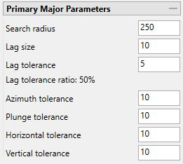
Search radius
The search radius should correspond to approximately half the distance of your data field. if the search radius is greater than the halfway point, then the search will over-extend the edge of the data.
If the distance traversing your sample area is 500 feet, then set the search radius to 250 feet.
Lag size
The lag size is the distance for each step from the origin. Set a lag size that coincides with your data spacing.
If your samples are spaced 50 feet apart, then set your lag size to 50. If you have to err, do so on the side of too small.
Lag tolerance
The lag tolerance is the distance plus or minus the lag size that samples will be captured. This helps capture samples that are not located at the exact distance interval as the lag spacing. Set the distance within which to use samples.
Note: If this is set to 0, then the tolerance is not used.
Samples are rarely located at exact intervals such as every 50 feet throughout the entire domain. There will nearly always be some variance. You can capture the samples that are not at exact intervals by setting the variogram to recognise samples that fall within 25 feet of the lag size, which in our sample case is every 50 feet.
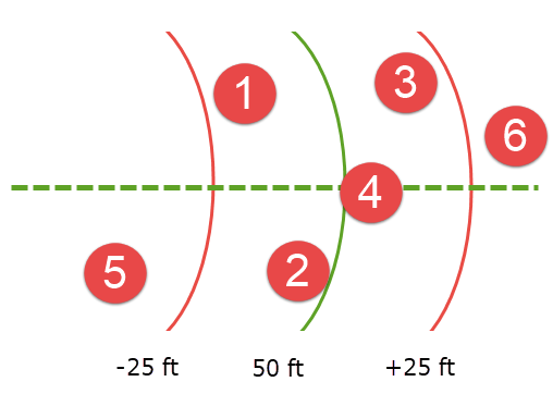
Here, the green line represents a lag size of 50 feet, and the red lines represent a lag tolerance of 25 feet on either side. Samples 1, 2, 3, and 4 would be used in the calculation. However, samples 5 and 6 would be ignored.
Lag tolerance ratio
This corresponds to the percentage of the lag size that is used by the lag tolerance.
A lag size of 50 with a lag tolerance of 25 will result in a lag tolerance ratio of 50%.
Azimuth tolerance
Enter the limit on the angle between two samples as measured in the plane of the plunge of the variogram.
Plunge tolerance
Enter the limit on the angle between two samples as measured in a vertical plane in the direction of the azimuth.
Note: A combination of cone, azimuth and plunge tolerances is used if the azimuth angle tolerance and plunge angle tolerance are set to less than the cone angle tolerance.
Horizontal tolerance
Enter the horizontal distance limit on sample pairs. Any acceptable sample must be within this horizontal distance of the centre of the variogram cone.
Tip: Set this value to a typical spacing (or larger) between your data, for example, if your data is on a 100 × 100 × 10 grid, set a horizontal distance of 100 and a vertical tolerance of 10. If you receive too few sample pairs, try increasing the tolerances to capture more data otherwise artifacts such as "hole effects" may occur.
Vertical tolerance
Enter the vertical distance limit on sample pairs. Any acceptable sample must be within this vertical distance from the centre of the variogram cone. The vertical distance is measured from the plane of the plunge of the variogram cone.
Unfolding
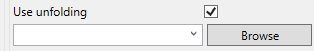
The unfolding option is used in the case of deformed strata bound deposits. This can be applied to deposits where mineralisation is controlled by a structural surface that can be modelled. The specification file from a Grid Model is used.
Indicators
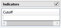
Enter the cutoff number that will become the threshold value. All values below the cutoff will be treated as 0, while all values equal to or above the cutoff will be treated as 1.
Chart Settings tab
Chart Titles
By default, the title is filled in with the <variable> + <direction>. However, you may enter your own title by replacing the default entry, or remove the title by deleting the text.
Gridlines
Select this option to display the gridlines at major intervals on the chart. You can elect to display gridlines for both axes or just one, depending on your needs.
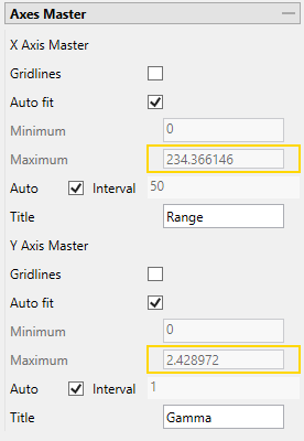
Auto fit
By default, Vulcan Data Analyser will auto fit the axes based on the values calculated from the dataset. However, you can customise the axes to highlight your particular study and needs. This can be done in two ways:
Method One
-
Deselect Auto fit.
-
Set a Minimum and Maximum range.
-
Let Vulcan Data Analyser adjust the intervals automatically by leaving the Auto Interval option selected.
Method Two
-
Deselect Auto fit.
-
Set a Minimum and Maximum range.
-
Deselect Auto Interval, then enter an interval of your choice.
Axes Titles
By default, the axes are provided with the traditional titles of Gamma and Range. However, if you wish to change these you may do so by replacing the text in each of the textboxes.
Annotations and Legend
Model tab
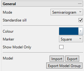
Mode
Note: The list of modes available for use depends on the type of variogram you are modelling. Depending on what type of variogram you are modelling, some of these modes might not be available.
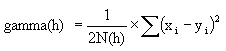
This is the standard semi variogram.
This is like the standard semi variogram, but divided by the mean of the data values.
This is like the standard semi variogram, but each difference is divided by the mean of the sample values.
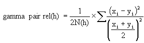
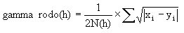
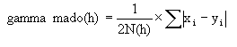
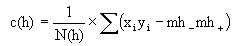
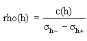
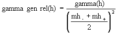
sqrt(Semivariogram) / Madogram
Transform data as 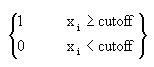 and compute the semivariogram
where:
Standardize sill
This option is disabled. You cannot set a standardised sill in a cross variogram.
Colour and Marker
Use the drop-down menus to select the colours and markers to customise the charts.
Show Model Only
Select this option to show only the model and hide the experimental variogram data.
Model Import / Export / Export Model Group
A model can be imported in or exported out. The files are stored as <filename>.vrg. The models that are exported out can be used in block model estimations.
Model Configuration
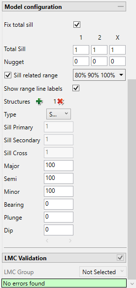
Fix total sill
Enabling this option prevents the sill from being changed when setting up the structure(s).
Total Sill
If you do not know the exact sill, enter a number that is close. Start with a whole number or a number rounded to 0.5 and work from there. The sill you choose will not affect the model calculations. It will only affect how you are able to see it on the chart.
The total sill is equal to the nugget plus all the structures such that
Total Sill = Nugget + Structure 1 + Structure 2 +... + Structure n
Nugget
You can enter the nugget obtained from the down hole variogram or enter another nugget. The default nugget is 0.
The nugget is the variance at an infinitely small separation distance.
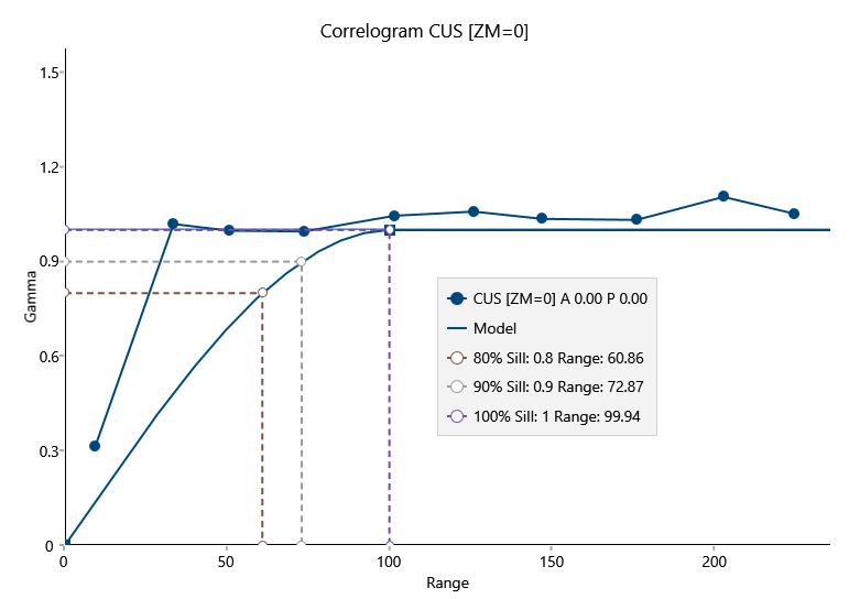
Sill related range
Use this option to add up to three vertical lines showing where the range would intersect the sill.
Show range line labels
Use this to display the legend for the range lines.
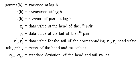
A variogram is a statistically-based, quantitative, description of the spatial correlation of sample points.
For each model the correlation function is described.
Note: On variography plots, the variance function, or maximum sill - correlation is plotted.
The representations below are in a single direction; however, in practice, models are always 3D and have shapes in any direction.
The 3D shape is controlled by a rotation (bearing, plunge, dip) and three ranges (major, semi, minor).
Nested
A nested variogram is a linear combination of several types of variograms allowing precise matching of sample behaviour. Up to 8 variograms can be nested in Vulcan.

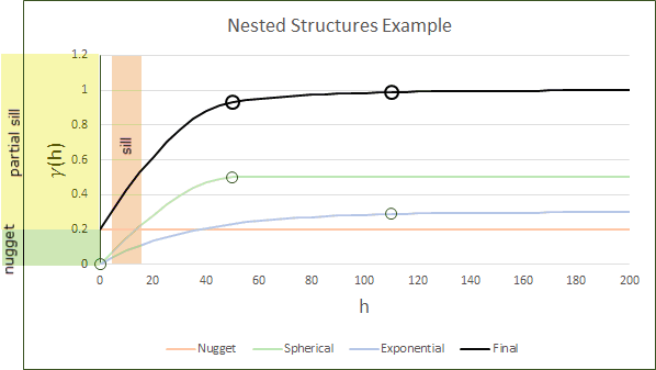
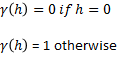
Nugget
The nugget is the variance at an infinitely small separation distance.
This type has no spatial correlation and should be a small component of the overall variance.
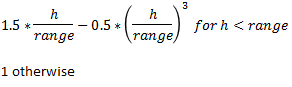
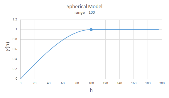
Spherical
This type is the most commonly used for ore deposits. They exhibit linear behaviour at and near the origin then rise rapidly and gradually curve off.

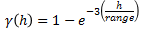
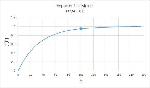
Exponential
This type is associated with an infinite range of influence. The sill is reached at the specified range parameter. Here the range parameter is found at 1/3 of the effective range.
For backward compatibility, see the Exponential3 Model.

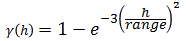
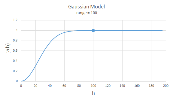
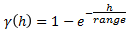
Gaussian
This type exhibits parabolic behaviour at the origin and, like the spherical model, rises rapidly. The Gaussian type reaches its sill smoothly, which is different from the spherical model, which reaches the sill with a definite break. The Gaussian model is rarely used in mineral deposits of any kind. It is used most often for values that exhibit high continuity.
To use this model, enter the effective range of the sill.
For backward compatibility, see the Gaussian3 Model.

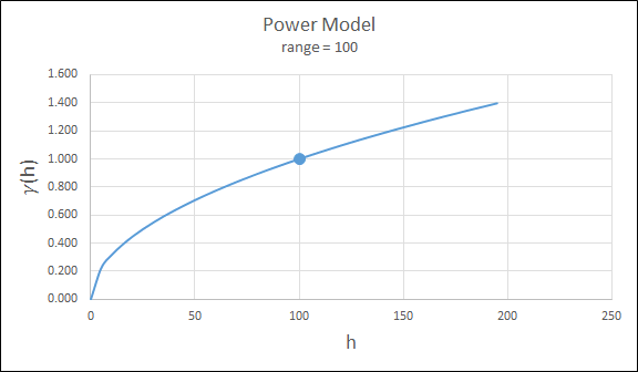
Power
For this model the major axis serves as the range parameter. The semi-major and minor axis distances must be adjusted in a corresponding ratio to preserve the anisotropy.

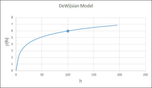
DeWijsian
This type is a representation of a linear semi-variogram versus its logarithmic distance.

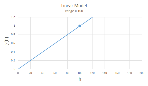
Linear
This type is a straight line with a slope angle defining the degree of continuity.
Note: that this model does not reach a sill.


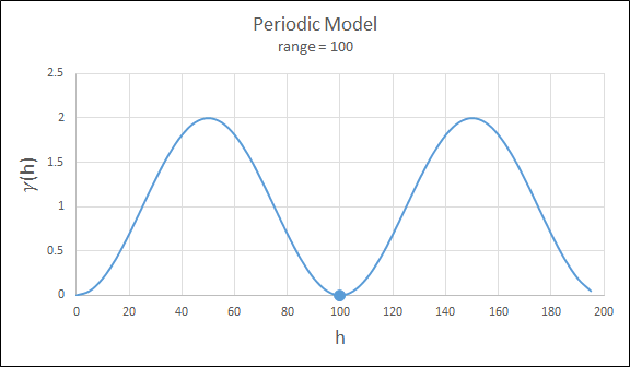
Periodic
This is a sine wave with one complete period over the effective range. This model is not commonly used because it can cause samples at greater distances to have higher correlation.

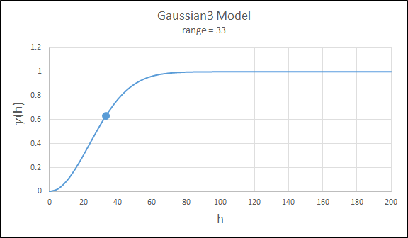
Gaussian3
This is just like the Gaussian model, but 3 times the effective range must be entered. This is for compatibility with previous releases.

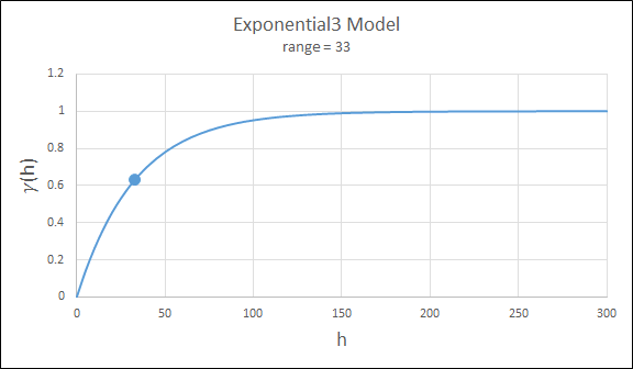
Exponential3
This is just like the exponential model, but three times the effective range must be entered. This is for compatibility with previous releases.

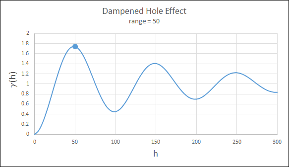
Dampened Hole Effect
Dampening is achieved by multiplying the covariance function by an exponential covariance, that acts as a dampening function.

LMC Validation
LMC Validation (Linear Model of Correlation) is required to use cokriging in non collocated data.
You can group variogram models to meet the LMC conditions by selecting the single variable models from the drop-down list.
LMC Validation requires that the single variable variograms are standardized and the cross variogram is not standardized.
Grouping models will synchronize the following model parameters:
-
Major
-
Semi
-
Minor
-
Bearing
-
Plunge
-
Dip
Therefore, changing these values in one of the models will update it in the whole group.
Note: The nugget and structure sill are not synchronized.
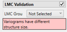
Messages indicating any errors will be displayed.
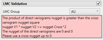
Important: For the nugget and the structure sill, the cross variogram value square must be lower or equal to the product of the direct variograms.
