Vulcan

Create Multiple Surfaces

Use the Create Multiple Surfaces option to create grid models based on existing mapfile data.

Instructions

On the Grid Calc menu, click Create Multiple Surfaces.

Load Specifications

Note: Desurvery information (if available) is used by default when generating grid surfaces through this tool.

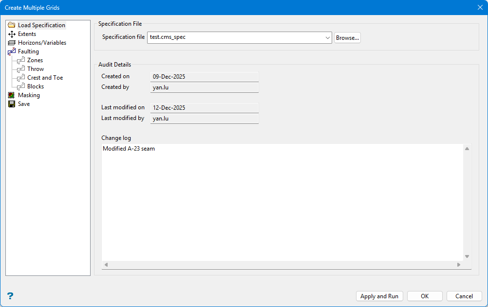
Specification file

Select the specification file (.cms.spec) that you want to open. The drop-down contains all of the .cms.spec files found in the current working directory. Click Browse if this file is not located in the current work area.

Audit details

These fields are automatically populated if the nominated specification file has any modification history. The Created on/by an Last modified on/by fields are read-only, and cannot be modified.

Buttons
Apply and Run	Click this button to save the entries before performing the compositing run. Once selected, the Coal Compositing interface will be hidden temporarily and the compositing run is performed. If a compositing run is cancelled, you will need to confirm that you want to interrupt the compositing run before the interface can be displayed again.
OK	Click this button to save all entries before exiting the Coal Compositing interface or moving to the next panel.
Cancel	Click this button to exit the Coal Compositing interface without saving any settings.

Extents

Note: Desurvery Information (if available) is used by default when generating grid surfaces through this tool.

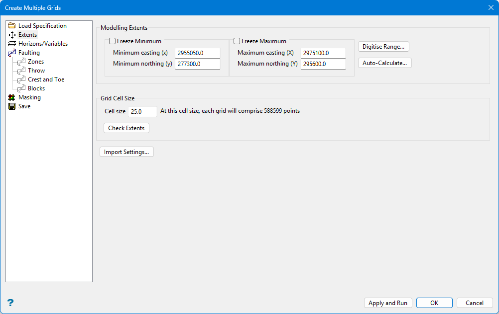
Coordinate Range

Specify the values for the minimum and maximum Eastings and Northings. These values define the four corners of every grid created using these specifications.

Note: The grid(s) cell size must divide evenly into the Easting and Northing extents of the area.

Freeze Minimum / Freeze Maximum

Select the Freeze Minimum or Freeze Maximum checkbox if you want the minimum or maximum extents to stay the same when the extents are recalculated.

Cell Size

Enter the Cell Size. After you enter a cell size and click Check Extents, the number of points that will make up the grid is re-calculated and displayed to the right of the box.

Check Extents

Click the Check Extents button to re-calculate extents.

Digitize Range

Click Digitize Range if you want to dynamically digitise the extents. Click on the desired minimum and maximum values to digitise the extents. When you return to the interface, the minimum and maximum fields contains the appropriate values.

Auto-Calculate

Note: To view the current extents, click Digitize Range. Once selected, the interface will "collapse" and the current extents will be displayed. Right-click to return to the interface.

Click Auto-Calculate if you want to use an existing drillhole database to calculate the X and Y extents. Once selected, the Auto Calculate Model Extents panel will be displayed.

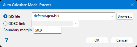
Select a drillhole database and specify the border margin. The drop-down list displays all drillhole database found within your current working directory.

Click OK to return to the interface.

Enter the default grid cell size. As a general rule, one-fifth of the average data spacing is a suitable size. While there are no software limits on the number of cells within a grid, obviously speed of operation may suffer when using a large numbers of cells. Grid cell size values can contain a single decimal place.

Import Settings

Click Import Settings if you want to use the settings contained within another file. Once selected, the Import Model Extents panel is displayed.

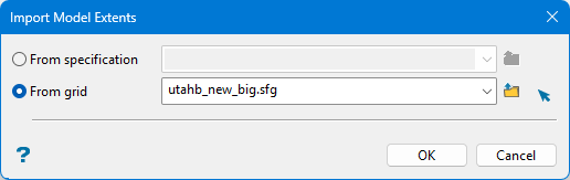
Specify the name of the specification file that contains the desired settings. The drop-down list displays all .gdc_spec, .fd_spec, .sme_spec and .cms_spec files found within your current working directory. Click Browse to select a file from another location.

Select the grid file (.sfg) from the drop-down list. The drop-down list displays all grid files found within your current working directory. Click Browse to select a file from another location.

Click OK to return to the interface.

Horizons/Variables

This panel may be pre-populated depending on the option you are using. If you have already made your mapfiles or mapbase, you can fill in this panel by clicking Populate and selecting the file.

You can copy, paste, insert, clear, or delete rows by right-clicking on the row number and selecting the appropriate option from the menu.

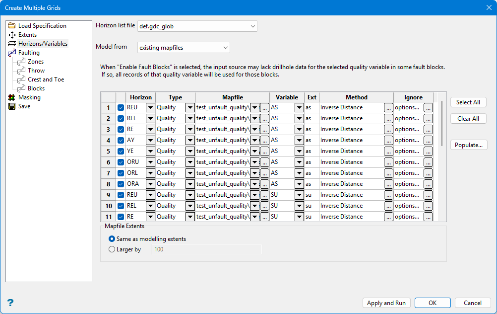
Horizon list file

Select a horizon list file from the drop-down list.

Model from

Select Existing mapfile or A mapfile database to specify which to use as a model for the surface.

Horizon

Select the horizon of interest from the drop-down list. (This option is only displayed if Existing mapfile is selected from the Model from list.)

Type

Select Structural or Quality from the drop-down list to specify the database type.

Mapfile

Select a mapfile from the list, or click "... " to select a file from another location.

Variable

Select the variable from the drop-down list. (This option is only displayed if Existing mapfile is selected from the Model from list.)

Ext

Enter the grid extension in the Ext field.

Method

Click "... " to display the Method panel to define the modelling method for the grid.

Modelling Method and Parameters

Select one of the following modelling algorithms

Triangulation

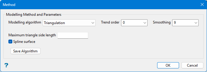
This method is typically used for modelling structural surfaces, such as structure roof and floor and structure thickness, and is recommended for modelling deposits with thin bedding planes. The results are a unique interpolated surface that honours all of the raw data values. Using a trend surface with this modelling method allows a regional feature to be applied to the local area of interest.

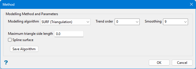
The triangles are as close to equilateral as possible and have a data point at each vertex. There will be linear interpolation between the three node points that make up each triangle. This method cannot extrapolate values higher or lower than the actual point values, causing the tops of hills and the bottoms of drainage areas to become flat. To avoid this scenario, the triangulation can be manipulated by applying a spline to the surface. The triangle network is covered with a mathematical surface that passes through each data point and is tangential to each point's previously determined slope, resulting in a surface that changes smoothly in all direction. All of the raw data values are honoured and the surface is projected above and below raw data values between data point locations.

This method does not allow for surface extrapolation beyond the raw data point locations. Vulcan uses Trending and Inverse Distance to extrapolate a triangulation to the model's edge.

Trend Order

Specify the triangulation trend order. Refer to the Trend option (in Grid Calc > Data ) for more information.

Smoothing

Specify the number of smoothing passes to be applied to the grid once it has been created. Smoothing applies a mathematical equation that calculates the variance of the modelled data. Once the value has not changed from the previously calculated variance by a certain percentage, the iterations or calculation process are discontinued. Usually nine smoothing passes are sufficient.

Spine Surface

Select this checkbox if you want to produce smooth grids without any smoothing when interpolating within the triangles. Breaklines are recognised.

Maximum triangle side length

Enter the maximum length for a triangle side. Grid points evaluated within a triangle with a side length greater than the specified length will have a data mask value of 0.

Save Algorithm

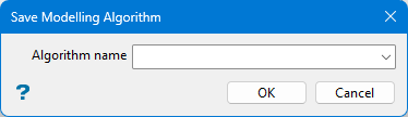
Select an algorithm name from the drop-down list, or enter a name for a new one.

Inverse Distance

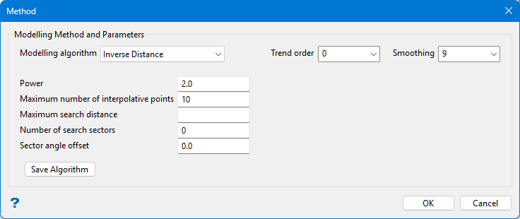
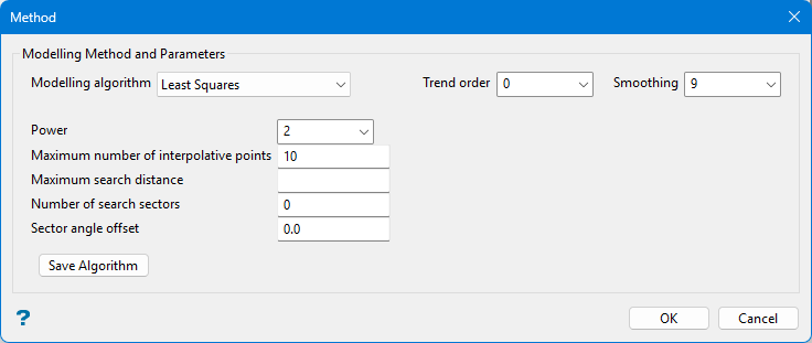
This method is typically used for modelling thickness and quality information. This method searches concentrically about each grid node for a minimum number of points to use to interpolate the grid node value. The number of points used and the distance to search for these points is specified as part of the method parameters. You can also divide the area into a maximum of 8 sectors, forcing the program to find the closest points in each sector, which is useful if the drillhole data is predominantly found in one section of the modelling area. This method should not be used on faulted datasets or for deposits where the bedding planes are thin.

The grid node values are determined by taking a weighted average of the collected data points. Therefore, the closer a drillhole is to the grid node, the greater the effect it will have on the calculated node value. The weighting used is the inverse of the distance to the nominated power.

Trend Order

Specify the triangulation trend order. Refer to the Trend option (in Grid Calc > Data ) for more information.

Smoothing

Power

Enter the inverse distance power (the default value is 2).

Maximum number of interpolative points

Specify the number of interpolative points to be used by the inverse distance method (the default value is 10).

Maximum search distance

Specify the maximum search radius for the inverse distance method. Grid points evaluated using points further than this distance from the grid point will have a data mask value of zero. The default is unlimited search distance.

Number of search sectors

Enter the number of search sectors (a maximum of 8). This option allows you to divide the search area into sectors so that data selected for modelling does not come from a cluster of points. Usually 8 sectors are used.

Sector angle offset

Enter an angle, in degrees, for the offset of the sectors. For example, if you choose to have 6 sectors and a sector angle offset of 0, then the first sector extends from a bearing of 0 to a bearing of 360 ÷ 6 (360 divided by 6)=60°. However, if the number of sectors is 6 and the sector angle offset is 5°, then the first sector extends from a bearing of 5° to a bearing of 60+5=65°. Rotating the sectors can stop samples being located on a boundary, which can cause problems as there is no way to determine into which sector a sample is placed if it is on a border.

Save Algorithm

Select an algorithm name from the drop-down list, or enter a name for a new one.

Krige

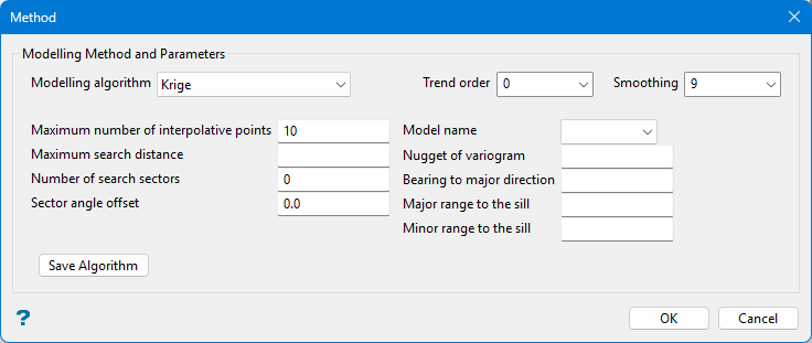
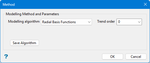
This method is based on a statistical analysis of spatially located data. The first step in kriging is to perform a variography analysis of the sample data. The resulting variograms express the degree of correlation between samples as a function of distance in several different directions. Sample data are usually correlated at short distances and less correlated at longer distances. Some sample data, such as water table levels, show a high degree of correlation at short distances. Other sample data, such as gold grade, usually show a larger degree of variance even at short distances. All sample data show a correlation approaching zero at larger distances. By fitting a variogram model function to the correlation data we make a function that predicts how well two samples will be correlated given their spatial relationship.

This method estimates a variable at a point by locating and weighting nearby samples. The weights take into account the degree of correlation between each sample and the estimation point, and also the degree of correlation between each pair of samples. The resulting weights provide a de-clustered weighting of the samples that minimises the variance as defined by the variogram.

Trend Order

Specify the triangulation trend order. Refer to the Trend option (in Grid Calc > Data ) for more information.

Smoothing

Maximum number of interpolative points

Specify the number of interpolative points to be used by the inverse distance method (the default value is 10).

Maximum search distance

Number of search sectors

Sector angle offset

Model name

Select the block model from the drop-down list.

Nugget of variogram

Enter the standardised nugget value returned from variogram analysis. The value returned (between 0 and 1) is the proportion of the variogram model sill represented by the variogram model nugget.

If the variogram model nugget value is '0.4', and the variogram model sill value is '2.0', then the nugget entered will be 0.4 ÷ 2.0 = 0.2.

The sill value does not need to be entered as its standardised value will be set as '1'.

The following fields define the shape and size of the variogram.

Bearing to major direction

Enter the bearing of the major axis of the ellipse.

Major range to the sill

Enter the length of the major axis. This is the distance from the centre of the ellipse to its edge in the major direction.

Minor range to the sill

Enter the length of the minor axis. This is the distance from the centre of the ellipse to its edge along the minor axis. The minor axis is perpendicular to the major axis.

If bearing = 90, major = 25 and minor = 15, then the ellipsoid is 50 long in the East/West direction, 30 wide in the North/South direction, and the major axis is parallel to the East/West axis.

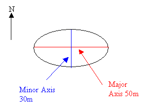
Figure 1: Example ellipse

If the bearing = 0, major = 25 and minor = 15, then the ellipsoid is 50 long in the North/South direction, 30 wide in the East/West direction, and the major axis is parallel to the north-south direction.

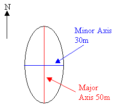
Figure 2: Example ellipse

Save Algorithm

Select an algorithm name from the drop-down list, or enter a name for a new one.

Spline

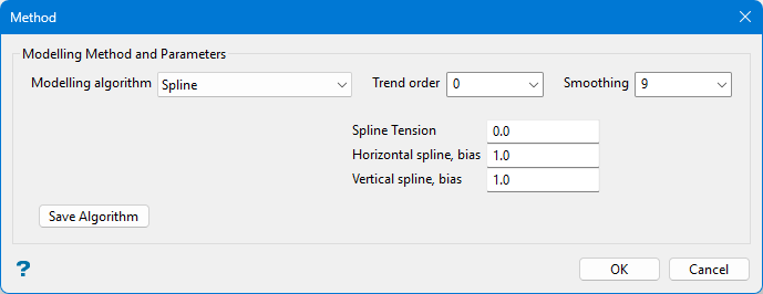
This method uses a drafter's spline, which is a flexible curve that can be fitted to a sequence of points so that a smooth curve can be drawn between them. The procedure fits a low order polynomial along the grid lines to all adjacent sets of points and from these it interpolates values at the grid points. The spline method demands that the data points lie on the grid lines where the X and Y values are multiples of the grid spacing. Normally, the spline method is used to model string data, such as contours. The tension of the splines may be specified (negative value implies relaxed) as can the bias applied to the splines in the X (vertical bias) and Y (horizontal bias) directions.

Trend Order

Specify the triangulation trend order. Refer to the Trend option (in Grid Calc > Data ) for more information.

Smoothing

Spline Tension

Enter the spline tension. A negative value relaxes (curves) the splines, therefore the higher the negative value the more relaxed the splines will be (they curve more). A positive value increases the spline tension, it makes the splines pull tight over the control points, reducing, for example, the height of the tops of hills and the depth of valleys. The values are usually in the range of 3 to 3, but they can be more or less.

Vertical spline bias

Enter the bias to be given to splines along the vertical grid lines over the horizontal grid lines. For each grid point, two values are interpolated, one based on the vertical spline, the other on the horizontal spline. The actual grid value is determined by averaging these values. The VERTICAL BIAS and HORIZONTAL BIAS values are used to weight the average vb/(ht+vb).

Horizontal spline bias

See Vertical bias for an explanation.

Note: For no bias, leave both the Vertical bias and Horizontal bias fields blank. To ignore one or the other, use 1 and 0 or 0 and 1 (if Horizontal bias is zero, then the horizontal splines are ignored). To give twice as much bias to the vertical splines as to the horizontal splines, use Vertical bias 2 and Horizontal bias 1. Multiplying the bias by a value has no affect, i.e. 2 and 1 is the same as 20 and 10. If you are modelling contour data, and most contours run East/West, you will want to use a high Vertical bias since the splines running North/South will have lots of control from the contour, while those running East/West will be almost parallel to the contours and hardly ever intersect them.

Save Algorithm

Select an algorithm name from the drop-down list, or enter a name for a new one.

Least Squares

This method is sometimes called a "moving average" because each node in the grid is estimated as the average of values from control points within a neighbourhood that is moved from grid node to grid node. First, all control points are located that reside within a specified neighbourhood around the grid node to be estimated. The values of these points approximately define a sloping plane or low order polynomial. Secondly, the equation of the plane is calculated and used to estimate the value of the grid node. The process of fitting a plane and evaluating it to estimate the surface is repeated for every node on the grid.

Trend Order

Specify the triangulation trend order. Refer to the Trend option (in Grid Calc > Data ) for more information.

Smoothing

Power

Enter the inverse distance power (the default value is 2).

Maximum number of interpolative points

Specify the number of interpolative points to be used by the inverse distance method (the default value is 10).

Maximum search distance

Number of search sectors

Sector angle offset

Save Algorithm

Select an algorithm name from the drop-down list, or enter a name for a new one.

Trend Surface

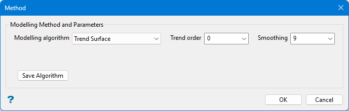
This method is based on the premise that small-scale features are masked and distorted in maps that are dominated by large scale, high amplitude features. Consequently, if the large-scale features are removed, then the smaller features are more easily identified and evaluated. This method applies a specified regional trend to the modelling process and then allows you to evaluate the residuals, or differences between the raw data values and the regional geological trend of the area.

First, a smooth regional map called a "trend surface" is made, this is a two dimensional global polynomial function. Then the differences between the original data point values and the smooth regional trend are calculated to produce a "residual" map (which displays the local features). Both maps may be significant in the geological interpretation.

Polynomials of degree 1, 2 and 3 are known as linear, quadratic, and cubic polynomials. A polynomial of degree 1 is a straight line if it is two dimensional or a plane if it is three dimensional. Every polynomial of degree 2 is a parabola with a vertical axis of symmetry that represents an anticlinal or synclinal shape. A third order polynomial defines an undulating surface. The third order trend may be applied to regional areas where both an anticline and an adjacent syncline are present or regions where the strata is actually folded. Higher order polynomials are not representative of geological surfaces. They tend to oscillate wildly between the outside control points and may generate very distorted values near the model's edge. How well the surface statistically fits the data can be determined from the "Goodness-of-fit" information produced during the modelling process.

Trend Order

Specify the triangulation trend order. Refer to the Trend option (in Grid Calc > Data ) for more information.

Smoothing

Save Algorithm

Select an algorithm name from the drop-down list, or enter a name for a new one.

EXIST (Inverse Distance)

Trend Order

Specify the triangulation trend order. Refer to the Trend option (in Grid Calc > Data ) for more information.

Smoothing

Power

Enter the inverse distance power (the default value is 2).

Maximum number of interpolative points

Specify the number of interpolative points to be used by the inverse distance method (the default value is 10).

Maximum search distance

Number of search sectors

Sector angle offset

Save Algorithm

Select an algorithm name from the drop-down list, or enter a name for a new one.

QUAL (Inverse Distance)

Trend Order

Specify the triangulation trend order. Refer to the Trend option (in Grid Calc > Data ) for more information.

Smoothing

Power

Enter the inverse distance power (the default value is 2).

Maximum number of interpolative points

Specify the number of interpolative points to be used by the inverse distance method (the default value is 10).

Maximum search distance

Number of search sectors

Sector angle offset

Save Algorithm

Select an algorithm name from the drop-down list, or enter a name for a new one.

SURF (Triangulation)

Spine Surface

Select this checkbox if you want to produce smooth grids without any smoothing when interpolating within the triangles. Breaklines are recognised.

Maximum triangle side length

Enter the maximum length for a triangle side. Grid points evaluated within a triangle with a side length greater than the specified length will have a data mask value of 0.

Save Algorithm

Select an algorithm name from the drop-down list, or enter a name for a new one.

THICK (Inverse Distance)

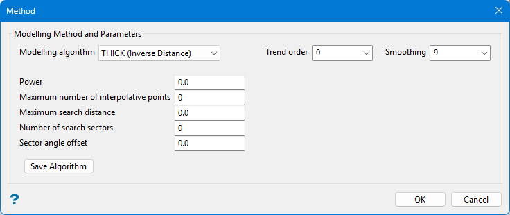
Trend Order

Specify the triangulation trend order. Refer to the Trend option (in Grid Calc > Data ) for more information.

Smoothing

Power

Enter the inverse distance power (the default value is 2).

Maximum number of interpolative points

Specify the number of interpolative points to be used by the inverse distance method (the default value is 10).

Maximum search distance

Number of search sectors

Sector angle offset

Save Algorithm

Select an algorithm name from the drop-down list, or enter a name for a new one.

Ignore

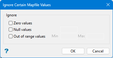
To ignore certain mapfile values, select the checkbox next to the appropriate option(s). You can specify a different set of rules for allowable values for each row.

Zero values

Ignore any mapfile values that are equal to zero.
Null values

Ignore any mapfile values that are equal to the null value that you specify in the box next to the Null values option.
Out of range values

Ignore any values that are below the minimum or above the maximum that you specify in the Min and Max boxes.

Mapfile Extents

The areal extent for the data gathered from the input mapfiles and CAD data are selected by default when a grid modelling range is selected. However, this option enables users to gather data from a wider area for use in calculating a model whilst still limiting the model's extent.

Same as modelling extents

Selecting this option enables user to limit the model's extents by the default value from mapfiles and CAD data.

Larger by

With this option, the model's limit is extended by a value (that is entered here) larger than the default value.

Zones / Throw / Crest and Toe

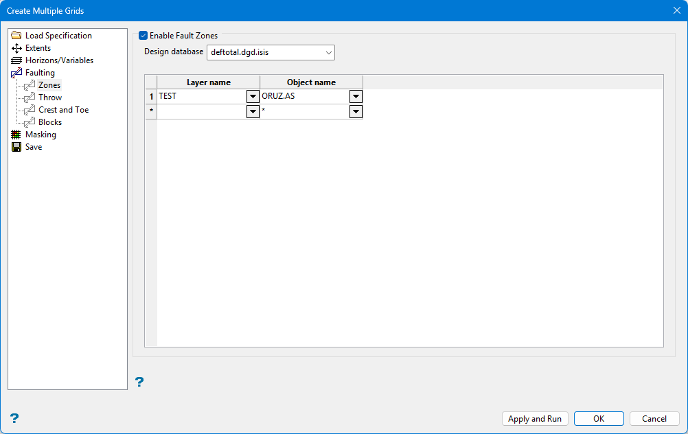
Enable Fault Zones

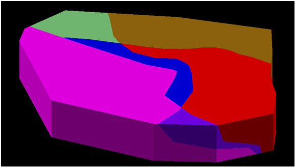
Select this checkbox if you want to create individual structural fault surfaces via a series of mutually exclusive polygons. The data present in each of the zones will be modelled independently within each polygon and the resultant patches of the grid model will be joined together at the polygon boundaries to form the final grid. Refer to Grid Calc > Faults > Load Fault Zones for more information.

You will need to specify the design database containing the zone polygons as well as the structural grid(s) that are to be faulted. The relevant layers and objects containing the zone polygons are then associated with each horizon.

Tip: A good way to create zone style polygons is to create an overall bounding polygon, then use the option Design > Polygon Edit > Build.

The available faulting options are not mutually exclusive.

Blocks

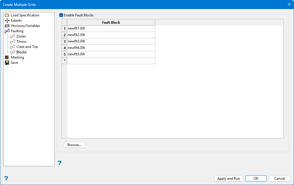
Enable Fault Blocks

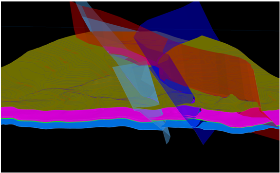
Select this checkbox if you want to use existing solid triangulations to define three-dimensional fault zones.To use a triangulation from an existing triangulation database, click Browse to locate the applicable triangulation database connection file (.tri). Once found, double-click on the file to display the Select Triangulation panel.

Click on the desired triangulation and then click OK.

The Input from existing map file checkbox, which is located under the Data Source(s) section, must be selected in order to access the available block faulting functionality. If this checkbox has not been selected, then all options displayed through the Blocks section will be disabled, i.e. unavailable.

You will need to enter the fault block names in the grid provided. We recommend that the names share a common "base name" with an identifying numeral, for example flt1, flt2, flt3. The solids must be:

valid closed solid triangulations
mutually exclusive.
cover the area of modelling data.
contain at least some data on any reference horizons specified.

The output will be a series of faulted surface triangulations named <proj><horizon>.srt and <proj><horizon>.sft (representing the roof and floor respectively). These triangulations are also gridded to provide faulted output grids, however, these grids will only represent normal faults whereas the triangulations will represent normal, reverse and thrust faults.

Masking

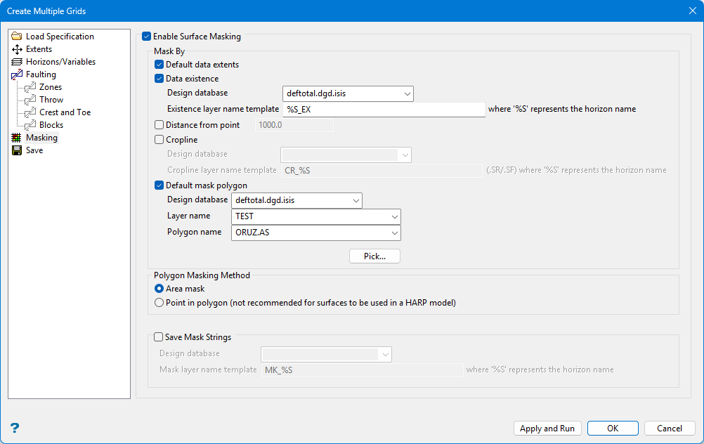
Enable Surface Masking

Select this checkbox to model all grids created to their full extent (as defined through the Extents section). If grid masking is required, then select the available checkbox.

Default data extents

Select this option to use the data extents you have set up in the dg1 parameters.

Note: Refer to Getting Started > Setting Up Vulcan > Creating a Project File (dg1) for more information.

Data existence

Select this option to use seam limit polygons for each horizon that have been created using GridCalc > Integrated Stratigraphic Modelling > Model Stratigraphy.

Distance from point

Select this checkbox to mask sections of the grid that fall beyond a nominated distance from known seam locations.

Cropline

Select this checkbox to use existing crop strings. You will need to select the design database containing the strings of interest as well as specify the naming template.

For example, if you have created a series of horizons named 'crop_<horizon>.SR' and 'crop_<horizon>.SF', then by entering 'crop_%S' the horizon name (sourced from the horizon list) will be automatically replaced in the layer name searched for.

Note: For a horizon named 'A' the cropping option will create resultant layers named 'CROP_A.SR' and 'CROP_A.SF' where the '%S' in the template name has been replaced automatically by the horizon name and the '.SR' and '.SF' represent the roof crop polygon and the floor crop polygon respectively.

Default mask polygon

Select this checkbox to supply a single layer and object combination which will be applied as a mask to all the horizons modelled, for example, a lease boundary. You will need to specify the design database, layer and polygon names. The specified layer must contain one or more polygons.

Click Pick to select a single default mask polygon directly from the screen. Once selected, the relevant information displays in the panel.

Note: As per grid modelling conventions, a clockwise polygon will be treated as an inclusion mask and an anticlockwise polygon will be treated as an exclusion mask.

Polygon Masking Method

Area Mask

Select this option to mask the four nodes that make up the grid cell if 50% of the cell area is included in the polygon. The cell is unmasked if more than 50% of the area is excluded by the polygon. The entire cell is taken into account. This option is the only method that considers a cell rather than individual nodes.

Point in Polygon

Select this option to mask a node if it is inside the polygon. Nodes outside the polygon are unmasked. Like masking from a grid, individual nodes are considered independent of the surrounding nodes.

Save mask strings

Select this checkbox to save the resultant overall mask strings created by the combination of any or all of the available mask generation options. The result will be the intersection of all the masks specified. As per previous layer saving options, a layer name for each horizon can be built up using a template whereby ‘ %S ’ represents the horizon name.

Save

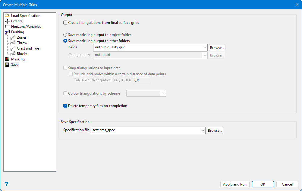
Output

Use this section to specify the storage location for the modelling output. You can choose to either save the output in the current working directory or in another location. When outputting to another location, the .tri and.grid folder extensions can be used to display the folder and its contents in the Vulcan Explorer application.

Note: We recommend that you store your grid output in your project folder, that is, your current working directory, to use the grids with other Grid Calc options.

Create grids from final surface triangulation or Create triangulations from final surface grids

Note: The Triangulations selection is only available if a Blocks or Throws with dips faulting method was defined.

If fault-blocking is specified, the Create grids from final surface triangulation checkbox is available.

If fault-blocking is not specified, the Create triangulations from final surface grids checkbox is available.

The naming convention applied to output grids or triangulations is important when creating a HARP model later.

If models were created without faulting, the grids are used to create the HARP model. Grids are named with the convention <proj><horizon>.srg or <proj><horizon>.sfg, where <proj> is the project prefix and <horizon> matches what is defined in the .gdc_blob file.
If models were created with fault throws which include dips, unclipped triangulations are used to create the HARP model. Triangulations are named with the convention <proj><horizon>.srg or <proj><horizon>.sfg, where <proj> is the project prefix and <horizon > matches what is defined in the .gdc_blob file.
If models were created with fault blocks, unclipped triangulations are used to create the HARP model. Triangulations are named with the convention <proj><horizon><fault block name>.srg or <proj><horizon><fault block name>.sfg, where <proj> is the project prefix, <horizon> matches what is defined in the .gdc_blob file, and <fault block name> matches the name of the input fault block triangulations.

Snap to input data

Select this option you wish to have the triangulation snapped to the data points.

Exclude grid nodes within a certain distance of input data

Select this option to enter a tolerance (distance) at which data points will be ignored.

Tolerance

Enter the distance at which data points will be ignored.

Specification file

The name of the currently open specification file, which was chosen through the Load Specification section, displays. The available drop-down list displays all .cms_spec files found in your current working directory. Click Browse to select a file from another location. Selecting an existing file will prompt you to confirm that you want to overwrite the file's original contents.

To create a new file, enter the file name and file extension.

Click Apply and Run to save the specification and create the surfaces.

Was this page helpful?