BM Normal Score

Use the BM Normal Score option to transform block model data from any distribution so that the transformed values follow a standard (normal) Gaussian distribution. The transformation is performed using the quantile transformation with a target distribution being a Gaussian standard. Unlike the Normal Score option, the transformation is performed using a nominated block model.

This option can also be accessed by selecting the BM Normal Score button from the Gaussian Transformations toolbar.

Instructions

On the Block menu, point to Gaussian Transformations, then click BM Normal Score.

Settings

Follow these steps:

Enter a name for the Specification file, or select it from the drop-down list. The drop-down list displays all files found in the current working directory that have the (.bmn) extension. Click the Browse icon to select a file from another location.
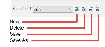
Select a Scenario ID. To create a new ID, click the New icon as shown below, and provide a unique name for the current panel settings.
Select the Block model from the drop-down list. Click the Browse icon to select a file from another location.
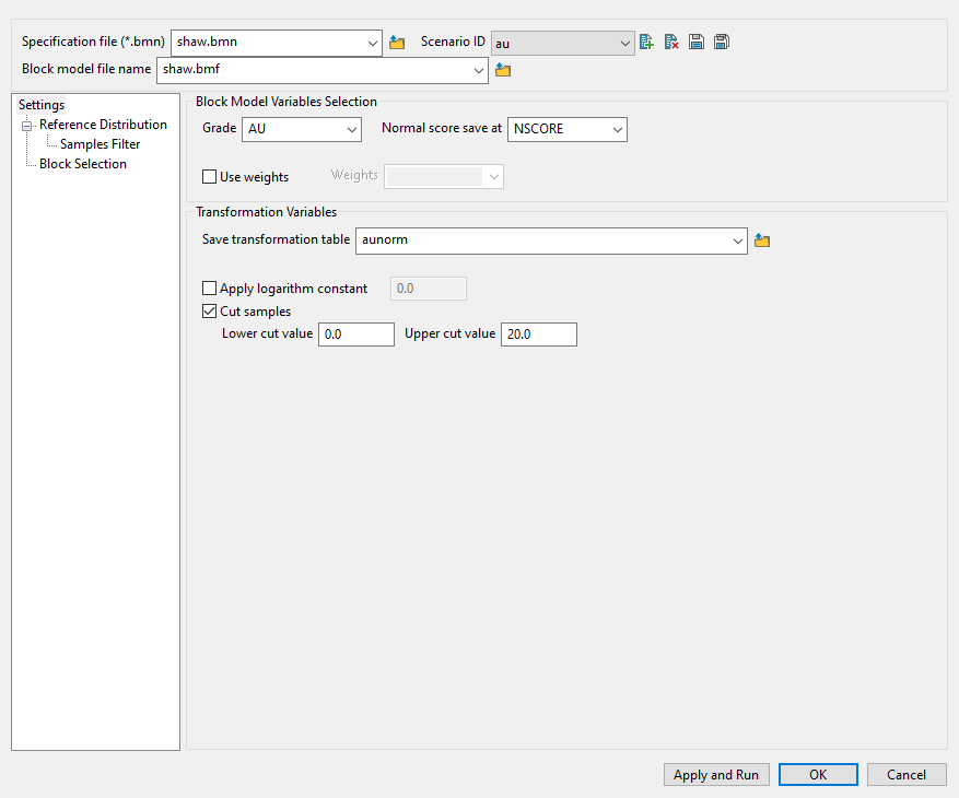
Map the correct fields by filling out the Block Model Variables Selection information.
1. Select the field containing the Grade values.
2. Select the block model variable that will hold the normal score values using the drop-down list labelled Normal score save at.
Enable Use weights to select the database field containing the weights that can be used to build the grade distribution. Sample values are not changed by the weighting, only the relative importance in the distribution is adjusted. Leave this field blank if you do not want to apply any weighting.
Enter or select a name for the file that will Save transformation table information.

This field refers to the lookup table with the correspondence between the grade value and it's associated Gaussian transformation. The specified transformation table will be created during the transformation process and its values will be stored in an ASCII mapfile. The resulting file can be used later to back transform Gaussian values into a block a model to the corresponding grade. Refer to the Normal Score Back option for more information.
Select Apply logarithm constant if you want to apply the base logarithm function to all values.

Important: In order for the logarithm to be defined all original values must be positive.

The specified logarithm constant will be added to the calculated logarithm.
Select Cut samples if you want to apply cut-offs to the values used in the transformation. You will need to specify a lower grade cut value (grades lower than this value are set to this value) as well as an upper grade cut value (grades above this value are set to this value).

Reference distribution

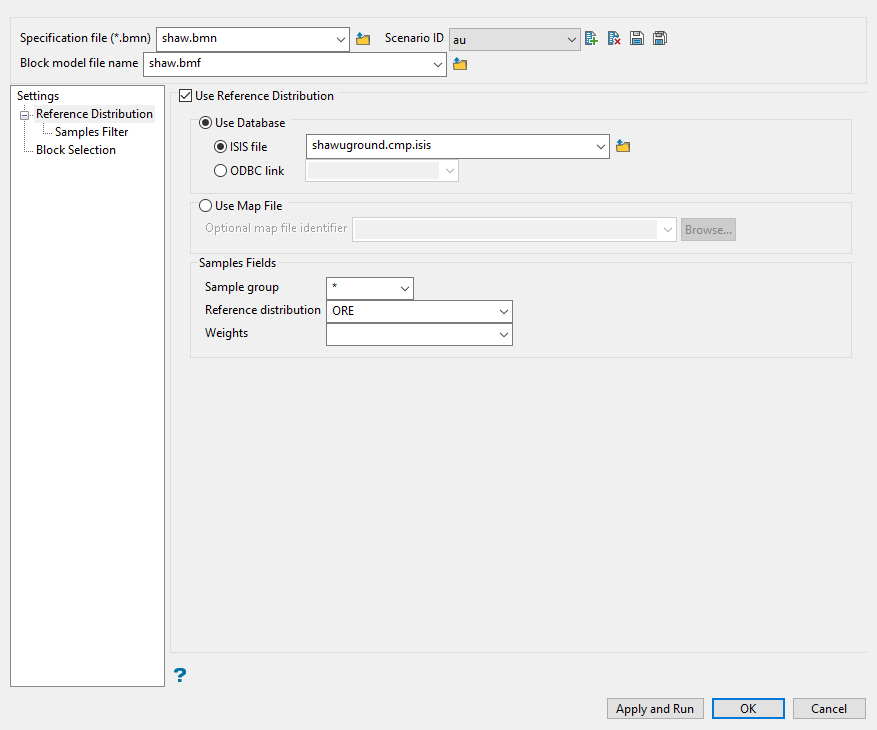
Use the Settings pane to define your specification file and scenario ID, as well as primary database information.

Follow these steps:

Select either a database or map file as your sample source.
- To select a database, enable the option ISIS file, then select the file from the drop-down list. Click folder icon to select a file from another location.
  
  You can also select an ODBC link for database files found on site servers.
- To select a map file, enable the option labelled Use Map File, then select the file from the drop-down list. Click the Browse button to select a file from another location.
Enter the name of the Sample Group to be loaded. Wildcards (* multi-character wildcard and % single character wildcard) may be used to select multiple groups. Multiple groups only apply to Isis databases (ASCII mapfiles consist of one group).
Select the grade variable that will be used to construct the transformation lookup table in the field labelled Reference distribution.
Select the database field containing the Weights that can be used to build the reference grade distribution. Sample values are not changed by the weighting, only its relative importance in the distribution is adjusted. Leave this field blank if you do not want to apply any weighting.

Samples Filter

Use this pane to include any restrictions to your data by using the four specialised filters.

Follow these steps:

Include any restrictions to your data by using the four specialised filters.
Select using Numeric tag
Use this filter to limit a numeric variable by only using specific values, ignoring specific values, or setting a range of values that can be used.

Follow these steps:
1. Enable this pane by selecting Sample Selection Using a Numeric tag.
2. Select the numeric field from the drop-down list.
3. Select Use specific numeric values to limit the values to only those listed in the table.
4. Select Ignore certain numeric values to create a list of values that will be ignored.
5. Select Use a numeric range to use all values found between a minimum and maximum threshold.
Note: You can use more than one filter. However, keep in mind that all conditions must be met for a value to be used.
Select using Character tag
Use this filter to limit a character variable by only using specific values or ignoring specific values.

Follow these steps:
1. Enable this pane by selecting Sample Selection Using a Character tag.
2. Select the Character field from the drop-down list.
3. Select Use specific character values to limit the values to only those listed in the table.
4. Select Ignore certain character values to create a list of values that will be ignored.
Note: You can use more than one filter. However, keep in mind that all conditions must be met for a value to be used.
Select using Solid triangulations
Use this filter to limit the samples by one or more triangulations.

Follow these steps:
1. Enable this pane by selecting Select using solid triangulations.
2. Add triangulations to the list by clicking the Browse or Screen Pick button.
  
  Clicking Browse will cause an Explorer panel to display.
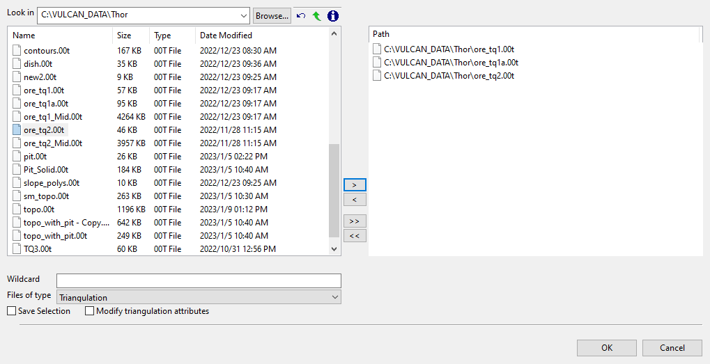
  Select Triangulation(s) panel
  
  Select the desired triangulation file(s) from the file list, which shows all available files in the current working directory. You can select files from a different location by clicking Browse..., or use the buttons to go to the last folder visited, go up one level, or change the way details are viewed in the panel, respectively.
  
  To highlight multiple list items at once, use the left mouse option in combination with the Shiftkey (this is for items that are adjacent in the list; for non-adjacent items, use the Ctrlkey and the left mouse option).
  
  Tip
  To filter file names using wildcard characters, type in a pattern in the Wildcard field using * for a multi-character and ? for a single-character wildcard.
  
  If you would like to use a previously created selection file (.sel) containing a list of desired triangulation files to load, choose Selection Files (*.sel) from the Files of type drop-down list.
  
  Move the items to the selection list on the right side of the panel.
  
  Click the button to move the highlighted items to the selection list on the right.
  
  Click the button to remove the highlighted items from the selection list on the right.
  
  Click the button to move all items to the selection list on the right.
  
  Click the button to remove all items from the selection list on the right.
  
  Select the Save Selection checkbox if you want to save the selection list (the right side of the panel), to a nominated selection file (.sel). Once this panel has been completed, a panel displays to save the selection file. Choose a selection file from the File Explorer to store the triangulation selection list to and click Save. To create a new file, enter the file name.
  
  Click OK to load the list of selected triangulations. Alternatively, click Cancel to close the panel without loading the selected triangulations.
3. Removing triangulations from the list by clicking the Clear Selected or Clear All button.
Select using Field restrictions
Use this filter to limit the samples to those with fields that match certain selection criteria.

Follow these steps:
1. Enable this pane by selecting Select selection using field restriction.
2. Select the field from the drop-down list in the Field column.
3. Enter the conditions that must be met in the Attributes column.
  
  Include spaces only if spaces are included in the desired field values.
  
  When entering a range, always enter the smallest number specified before the largest number.
  
  -792&-720 since -792 is smaller than -720. This range is evaluated as -792.0 ≤ VALUE < -720.0.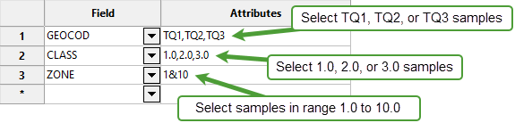
  
  Note: You can enter more than one condition. However, keep in mind that all conditions must be met for a value to be used.

Block Selection

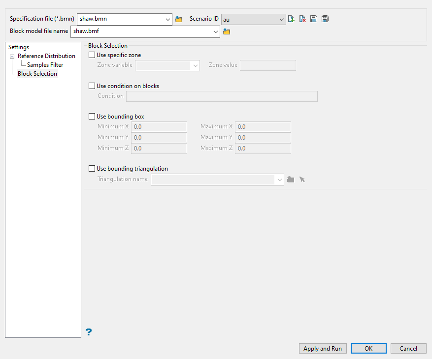
Use this panel to set up various block selection options.

Follow these steps:

Enter the maximum number of previously simulated grid nodes that will be used together with sample information in order to simulate block model nodes in the Maximum of presimulated blocks field. If the samples were not assigned to nodes through the Simulation parameters section, then the maximum number of samples will be controlled by the parameters specified through the Search region section.

If the samples were assigned to nodes, then the parameter specified at the sample counts are ignored and the maximum number of presimulated block nodes will apply to samples (already assigned to nodes) and nodes populated by simulation.
Select Use random search path to simulate the nodes in a random order.
Select Use multiple search grid path to perform a grid ordering as a first step before going into the random path. The grid refinement begins by simulating the nodes at a coarse regular grid spacing. The coarse grid spacing can then be further refined to half of the previous spacing.

Note: A maximum number of 4 consecutive grid refinements can be requested in the Number of grids field. After the regularly spaced nodes are simulated the remaining nodes are selected using a random path.

Select any of the options to limit the blocks used.

Was this page helpful?