Cube Editor
Use the Cube Editor option for a different way of computing and displaying variography data. Instead of computing variography in radially defined cones, the variography is computed in cubes. For each sample data pair, the difference vector is taken and the variography information for the cube in which the head of the vector lies is updated. The variography is written into a block model.
The block model is located around the origin in variography coordinates. You can display a block model of variography data using the usual block model display tools. For example, you can slice the block model, contour the block model, or load individual blocks with various colour schemes. The only requirement is that you create a Vulcan view of the space around the origin. The display of the variography block model gives a true three dimensional view of the variance of your data. You can also display the sill ellipsoid over the block model to see how well the ellipsoid matches the continuity in the variography data. The format of the block model file name is:
<proj><bfi>_vrs.bmf
Also generated is an associated _vrs.bdf file (block definition file). See Appendix A for an example the _vrs.bdf file.
Instructions
On the Block menu, point to Variography, then click Cube Editor.
Follow these steps:
-
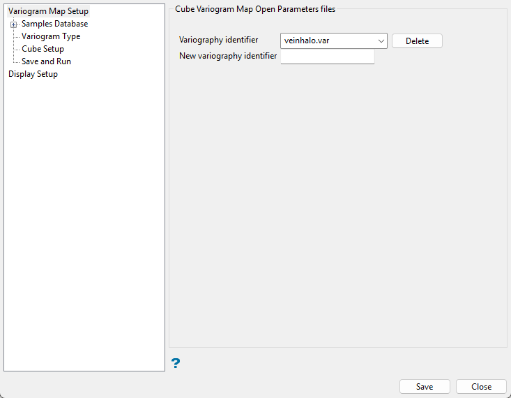
Select the Variography identifier or enter a new variography identifier. This is the name of an existing variography parameter file.
You can create a new identifier by entering the name of the new parameter file in New variography identifier. The maximum size is 10 alphanumeric characters.
Samples Database
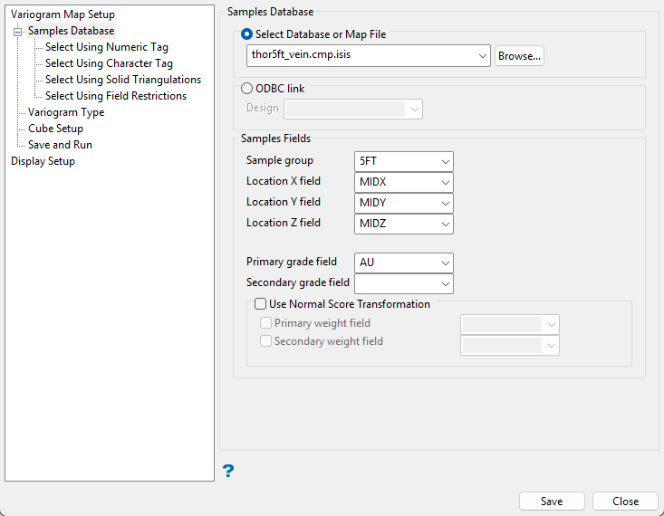
Use this section of the interface to select the database and database fields that will be used to generate the variograms.
Follow these steps:
-
Select either a database or map file as your sample source.
-
To select a database, enable the option ISIS file, then select the file from the drop-down list. Click folder icon to select a file from another location.
You can also select an ODBC link for database files found on site servers.
-
To select a map file, enable the option labelled Use Map File, then select the file from the drop-down list. Click the Browse button to select a file from another location.
-
-
Map the correct fields by filling out the Samples Fields information.
-
Sample group - Enter the name of the groups (database keys) to be loaded in the field. Wildcards (* multi-character wildcard and % single character wildcard) may be used to select multiple groups. Multiple groups only apply to Isis databases (ASCII map files consist of one group).
-
Select the names of the fields containing the X, Y, and Z coordinates in the Location fields.
-
Select the name for the variable containing the Grade values.
-
-
Include any restrictions to your data by using the four specialised filters.
 Select using Numeric tag
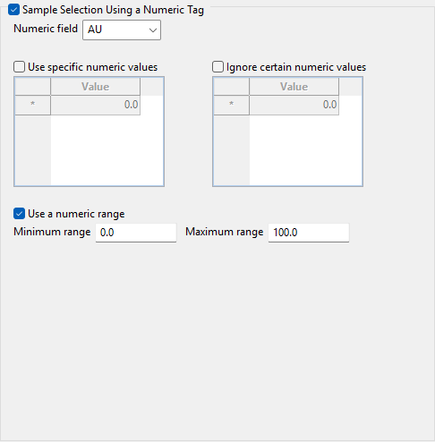
Use this filter to limit a numeric variable by only using specific values, ignoring specific values, or setting a range of values that can be used.
Follow these steps:
-
Enable this pane by selecting Sample Selection Using a Numeric tag.
-
Select the numeric field from the drop-down list.
-
Select Use specific numeric values to limit the values to only those listed in the table.
-
Select Ignore certain numeric values to create a list of values that will be ignored.
-
Select Use a numeric range to use all values found between a minimum and maximum threshold.
Note: You can use more than one filter. However, keep in mind that all conditions must be met for a value to be used.
Select using Character tag
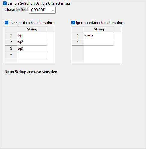
Use this filter to limit a character variable by only using specific values or ignoring specific values.
Follow these steps:
-
Enable this pane by selecting Sample Selection Using a Character tag.
-
Select the Character field from the drop-down list.
-
Select Use specific character values to limit the values to only those listed in the table.
-
Select Ignore certain character values to create a list of values that will be ignored.
Note: You can use more than one filter. However, keep in mind that all conditions must be met for a value to be used.
Select using Solid triangulations
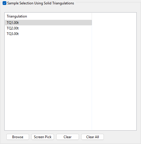
Use this filter to limit the samples by one or more triangulations.
Follow these steps:
-
Enable this pane by selecting Select using solid triangulations.
-
Add triangulations to the list by clicking the Browse or Screen Pick button.
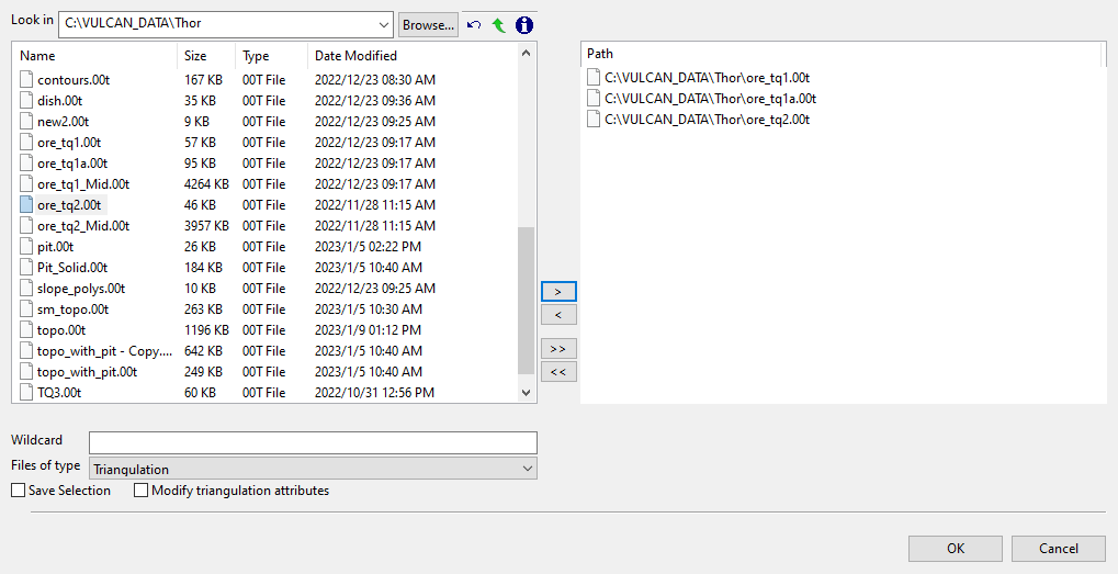
Clicking Browse will cause an Explorer panel to display.
Select Triangulation(s) panel
-
Select the desired triangulation file(s) from the file list, which shows all available files in the current working directory. You can select files from a different location by clicking Browse..., or use the
 buttons to go to the last folder visited, go up one level, or change the way details are viewed in the panel, respectively.
To highlight multiple list items at once, use the left mouse option in combination with the Shiftkey (this is for items that are adjacent in the list; for non-adjacent items, use the Ctrlkey and the left mouse option).
TipTo filter file names using wildcard characters, type in a pattern in the Wildcard field using
*for a multi-character and?for a single-character wildcard.If you would like to use a previously created selection file (.sel) containing a list of desired triangulation files to load, choose Selection Files (*.sel) from the Files of type drop-down list.
-
Move the items to the selection list on the right side of the panel.
- Click the
 button to move the highlighted items to the selection list on the right.
 - Click the
 button to remove the highlighted items from the selection list on the right.
 - Click the
 button to move all items to the selection list on the right.
 - Click the
 button to remove all items from the selection list on the right.
- Click the
-
Select the Save Selection checkbox if you want to save the selection list (the right side of the panel), to a nominated selection file (
.sel). Once this panel has been completed, a panel displays to save the selection file. Choose a selection file from the File Explorer to store the triangulation selection list to and click Save. To create a new file, enter the file name. -
Click OK to load the list of selected triangulations. Alternatively, click Cancel to close the panel without loading the selected triangulations.
-
-
Removing triangulations from the list by clicking the Clear Selected or Clear All button.
Select using Field restrictions
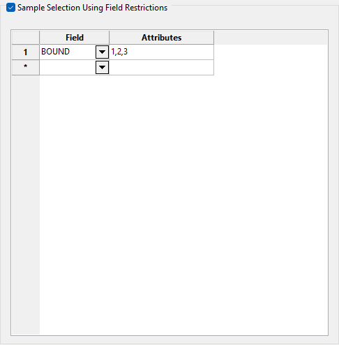
Use this filter to limit the samples to those with fields that match certain selection criteria.
Follow these steps:
-
Enable this pane by selecting Select selection using field restriction.
-
Select the field from the drop-down list in the Field column.
-
Enter the conditions that must be met in the Attributes column.
Include spaces only if spaces are included in the desired field values.
When entering a range, always enter the smallest number specified before the largest number.
-792&-720since-792is smaller than-720. This range is evaluated as-792.0 ≤ VALUE < -720.0.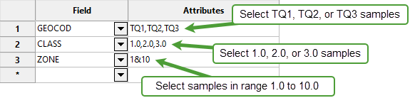
Note: You can enter more than one condition. However, keep in mind that all conditions must be met for a value to be used.
-
-
Enable Use normal score transformation to use transformed data.
-
Primary Weight Field - Enter the name of the grade variable.
-
Secondary Weight Field - Enter the name of the second grade variable. This should only be entered for cross-variography.
-
Use this pane to include any restrictions to your data by using the four specialised filters.
Variogram Type
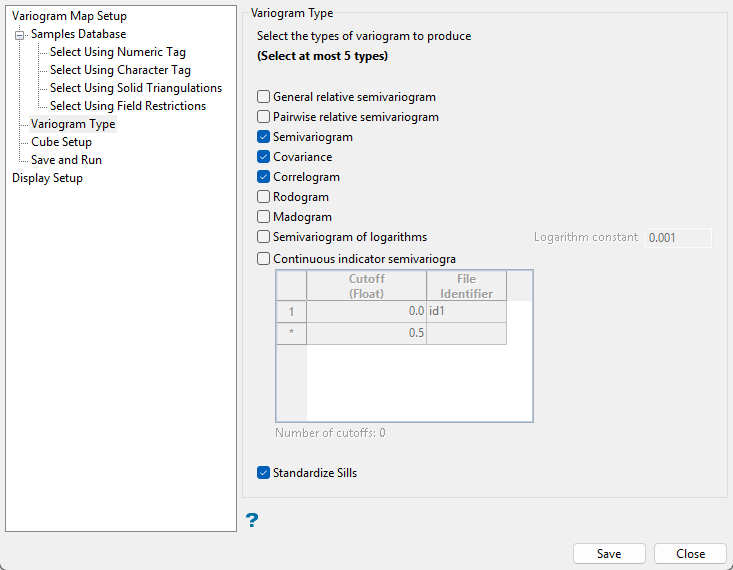
Follow these steps:
-
Select up to 5 variogram types.
-
Enable Standardise sill if you want to standardise the variogram sill by dividing the results by the sample variance. This is useful when calculating a semivariogram because instead of reaching the sill at the sample variance it will reach it at 1.
This is like the standard semi variogram, but divided by the mean of the data values.
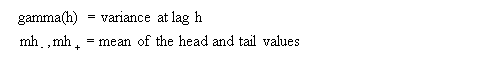
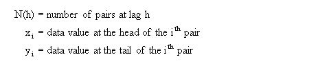
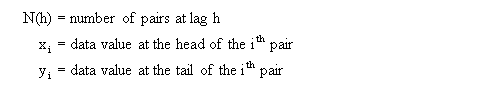
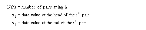
where:
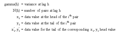
This is like the standard semi variogram, but each difference is divided by the mean of the sample values.
where:
This is the standard semi variogram.
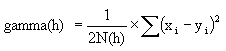
where:
where:
![]()
where:
where:
![]()
where:
where:
![]()
where:
Transform data as 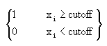 and compute the semivariogram.
where:

Cube Setup
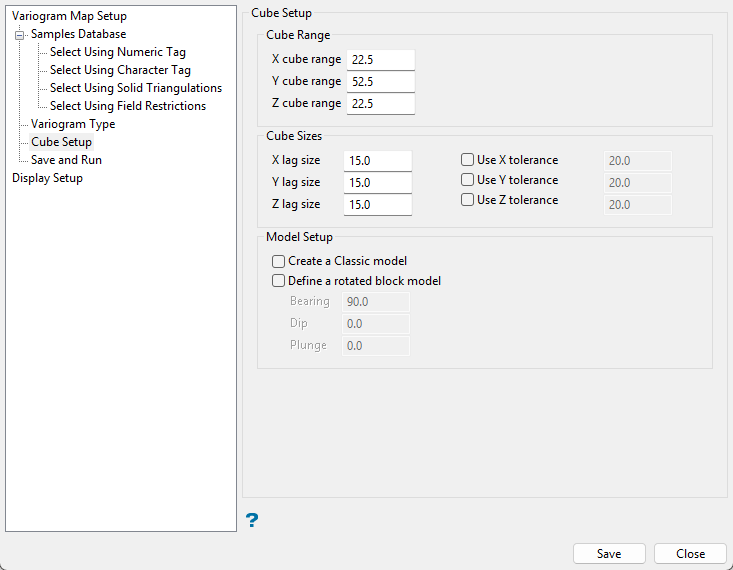
Follow these steps:
-
Enter the X/Y/Z cube range. This is the cube size and represents the variogram range in each of the X, Y, and Z directions.
-
Enter the X/Y/Z lag size. The lag size is the distance for each step from the origin. Set a lag size that coincides with your data spacing.
Example: If your samples are spaced 50 feet apart, then set your lag size to 50. If you have to err, do so on the side of too small.
Using a large lag distance puts more sample pairs into each block, but reduces the resolution.
-
As an option, you can enable Use X/Y/Z tolerance if you want to set a lag tolerance.
The lag tolerance is the distance plus or minus the lag size that samples will be captured. This helps capture samples that are not located at the exact distance interval as the lag spacing.
Note: If this is set to 0, then the tolerance is not used.
ExampleSamples are rarely located at exact intervals such as every 50 feet throughout the entire domain. There will nearly always be some variance. You can capture the samples that are not at exact intervals by setting the variogram to recognise samples that fall within 25 feet of the lag size, which in our sample case is every 50 feet.
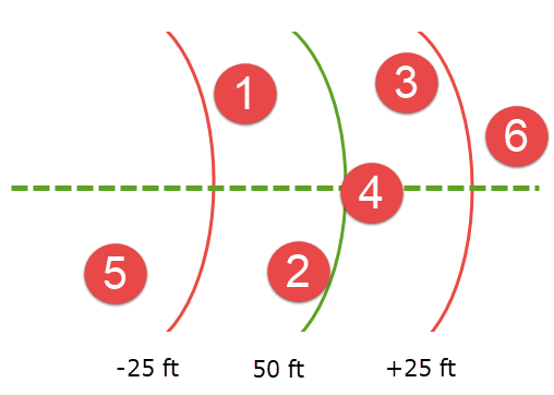
Here, the curved green line represents a lag size of 50 feet, and the red lines represent a lag tolerance of 25 feet on either side. Samples 1, 2, 3, and 4 would be used in the calculation. However, samples 5 and 6 would be ignored.
-
Enable Create a Classic model if you wish to create a new block model in the classic format. The new variography block model gives a true three-dimensional view of the variance of your data. You can also display the sill ellipsoid over the block model to see how well the ellipsoid matches the continuity in the variography data. The format of the block model file name is
<proj><bfi>_vrs.bmf, and will be stored in the Block Models folder. -
By default, there is no rotation given to the new model. To enter rotation parameters, click Define a rotated block model to enable the settings the for Bearing, Dip, and Plunge.
Display Setup
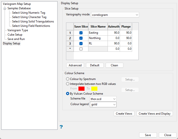
Follow these steps:
-
Use the Variography mode drop-down list to select the type of variography to display. The following variography types are available:
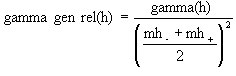
General relative semivariogram
This is like the standard semi variogram, but divided by the mean of the data values.
where:
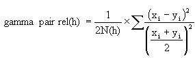
Pairwise relative semivariogram
This is like the standard semi variogram, but each difference is divided by the mean of the sample values.
where:
Semivariogram
This is the standard semi variogram.
where:
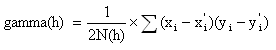
Cross-semivariogram
where:
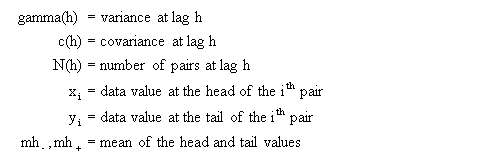
Covariance
where:
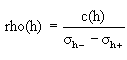
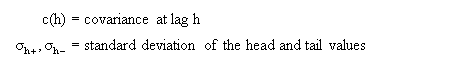
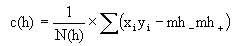
Correlogram
where:
Rodogram
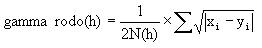
where:
Madogram
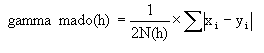
where:
Semivariogram of logarithms
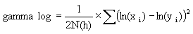
where:
Indicator semivariogram
Transform data as
and compute the semivariogram.where:
-
Check the Save Slice box to save the resulting slice. You will need to specify a slice name. The slice name can be up to 20 alphanumeric characters in length (no spaces). The
.00tfile extension is automatically added. If the check box is not checked, then the slice is generated and displayed as an underlay and deleted upon exiting Vulcan.The image registration and image files, which are automatically created when generating the resulting slice, will be named using the specified slice name.
Example: If you specified a slice name of AU_SLICE, then the resulting image registration and image files are named AU_SLICE.ireg and AU_SLICE.tiff.
Buttons
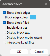
Advanced - Allows you to set additional display settings using the following panel.
Default - Loads setting parameters for three orthogonal views at 90 degrees to each other.
Clean - Removes all entries from the table.
-
Select the colour scheme.
Colour by Spectrum
Select this option to colour the slices by spectrum. This mean that the colour spectrum is stretched over the variable values, thus small variable values are represented by red, large values by violet and the largest by white, as shown in the diagram below:
 Interpolate between two RGB values
Select this check box the stretch two colour over the variable values.
Example: If you selected red and blue, then the small values would be red, the middle values purple and the large values blue. The colour of the middle values is an average of the two chosen colours, as shown in the diagram below:
 By Vulcan Colour Scheme
Select this check box to colour the slices using a Vulcan colour scheme. A default scheme file and type is entered automatically, these can be altered. Select the file, type and colour legend from the drip-down lists.
The colour schemes can be edited using the Analyse > Legend Editor option.
-
If you select a Device_Colour scheme type, the range of colours will be stretched over the variable values, similar, but not the same as, the Colour by Spectrum option.
-
Alpha legends are not fully supported.
Click Save and Run in the menu tree to calculate the variograms.
Note: This section does not contain any panel options.
Each time Save and Run is clicked, a confirmation prompt displays. Select Yes to perform the variogram calculation, or No to return to the interface.
Note: Select Do not ask me again to bypass the confirmation prompt and perform the variogram calculation automatically.
The results file will be stored in your current working directory and will be named using the following naming conventions:
<proj><file Id><parameter d>_prm.vrs
Click Save to save all the parameters and close the panel.
Click Close to close the panel without saving.
