Multi-Gaussian Simulation
Use this option to create a simulation based on Multi-Gaussian kriging.
Instructions
On the Block menu, point to Simulation, then click Multi-Gaussian Simulation.
Simulation Parameters
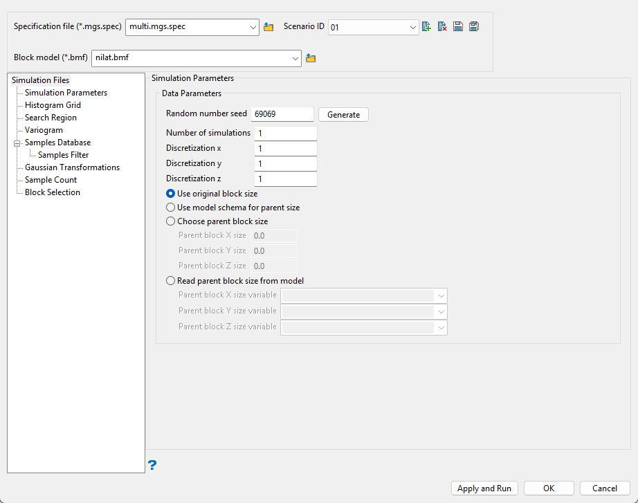
Follow these steps:
-
Enter a name for the Specification file, or select it from the drop-down list. The drop-down list displays all files found in the current working directory that have the (
.mgs.spec) extension. Click the Browse icon to select a file from another location.
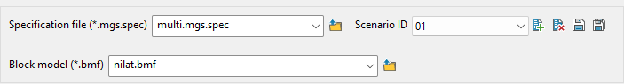
-
Select a Scenario ID. To create a new ID, click the New icon as shown below, and provide a unique name for the current panel settings. Up to nine separate IDs can be created for each
.mgs.specfile.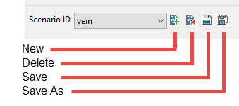
-
Select the Block model from the drop-down list. Click the Browse icon
to select a file from another location. -
Set the Random number seed. This is a parameter to initialise the random number generator in Vulcan. The random numbers are used for the random path and for drawing from the conditional distribution.
-
Enter the Number of simulations (or realisations) you want to perform.
TipHow many realizations should one draw?
The answer is definitely more than one to get some sense of the uncertainty. If two images, although both a priori acceptable, yield widely different results, then more images should be drawn. The number of realizations needed depends on how many are deemed sufficient to model (bracket) the uncertainty being addressed. Note that an evaluation of uncertainty need not require that each realization cover the entire field or site: simulation of a typical or critical subarea or section may suffice. (Deutsch, Journel, 1997)
-
Enter the Discretization steps in all three directions.
-
Select the block size to be used.
Tip: If after declustering your data, the sample spacing does not allow you to set up a block size small enough to represent the SMU, you can set up the discretization steps sizes to approximate the SMU.
-
Use original block size - Use this option if you are using a model with a sub-block scheme.
-
Use model schema for parent size - Use just the parent block size designated in the block definition file, ignoring any sub-blocks.
-
Choose parent block size - Enter a custom parent block size.
-
Read parent block size from model - Read the parent block size directly from the model.
-
Histogram Grid
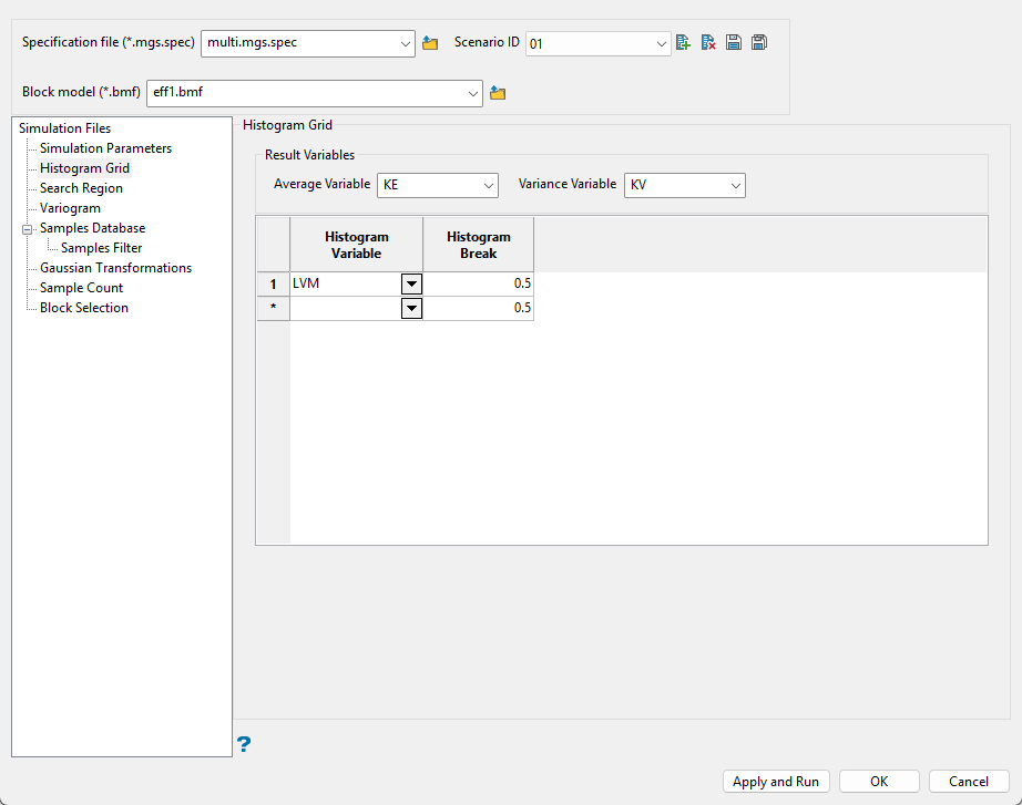
Follow these steps:
-
Select the Average Variable from the drop-down list. This is mandatory and is the block model variable that stores the average values.
-
Select the Variance Variable from the drop-down list. This is optional and is the block model variable that stores the variance.
-
You can select any number of Histogram Variables. Graphs will be produced for each variable.
-
Enter the Histogram Break. This is the size of each bin.
Search Region
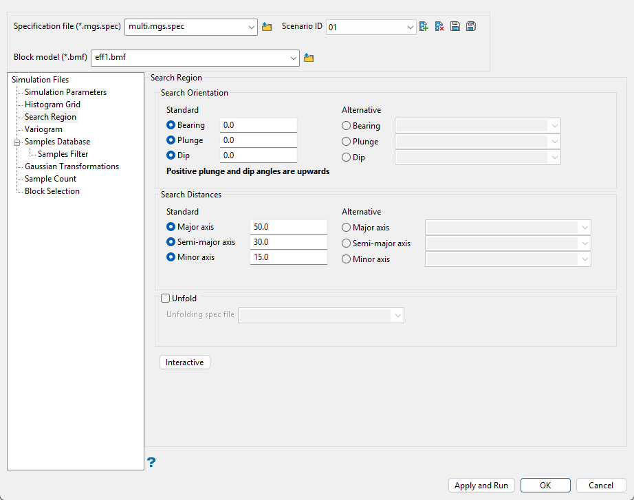
Use this pane to define the search distances and search orientation.
Follow these steps:
-
Enter the angles for the Bearing, Plunge, and Dip.
Note: You can enter the angles directly or select block model variables that contain the angles by choosing the Alternative options.
 Search Orientation
The Bearing, Plunge and Dip values are angles, in degrees, that specify the orientation of the search ellipsoid and orientation of variogram structures. Care must be taken with these parameters as there are several common misunderstandings about the meaning of these parameters.
To understand these parameters, imagine an ore body with a primary axis. To find the bearing of the ore body, project the ore body axis straight up onto the surface plane and call this line the bearing line. The bearing is the angle clockwise from north to the bearing line.
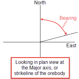
Figure 1: Bearing
Plunge is the angle between the horizontal plane and the ore body axis. Note that the plunge should be negative for a downward pointing ore body.
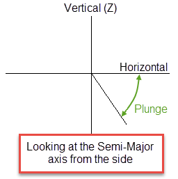
Figure 2: Plunge
To find the dip of an ore body, imagine the ore body is located in a plane. First rotate around the Z axis by the bearing so that the ore body is pointing north. Then rotate around the east-west axis by the plunge so that the ore body is level with the ground. At this point the ore body is parallel to the north-south axis. The dip is the angle of rotation to bring the plane into the horizontal plane. Looking north, if the plane must be rotated clockwise around the north-south axis, then the dip is positive (other software packages may use the opposite convention).
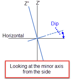
Figure 3: Dip
Note: The terms bearing, plunge and dip have been used by various authors with various meanings. In this panel, as well as kriging and variography, they do not refer to true geological bearing, plunge and dip. The terms X', Y' and Z' axis are used to denote the rotated axes as opposed to X, Y and Z which denote the axes in their default orientation.
-
Enter the dimensions of the search region.
Search Distances
The search box has sides with length twice the numbers given. The major axis radius is the search distance along the axis of the ore body. The semi-major radius is the search distance in the ore body plane perpendicular to the ore body axis. The minor axis radius is the search distance perpendicular to the ore body plane.
Note: Use the Display Ellipsoid option to verify that you are using the proper orientation angles. Display the search ellipsoids over your sample data to verify the correct orientation of the ellipsoid.
The search radii are true radii. If you set your major search radius to '100', then the ellipsoid has a total length of 200. The following diagram shows the relationship between the axes with the ellipse in the default orientation (bearing 90°, plunge and dip 0.00°).
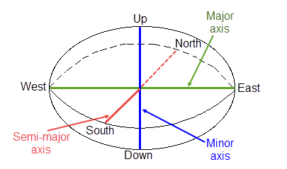
Figure 4: Relationship between Radii
-
Select Unfold to use a tetrahedral model. This is applicable only for folded or faulted block models for which a tetrahedral model has been created.
-
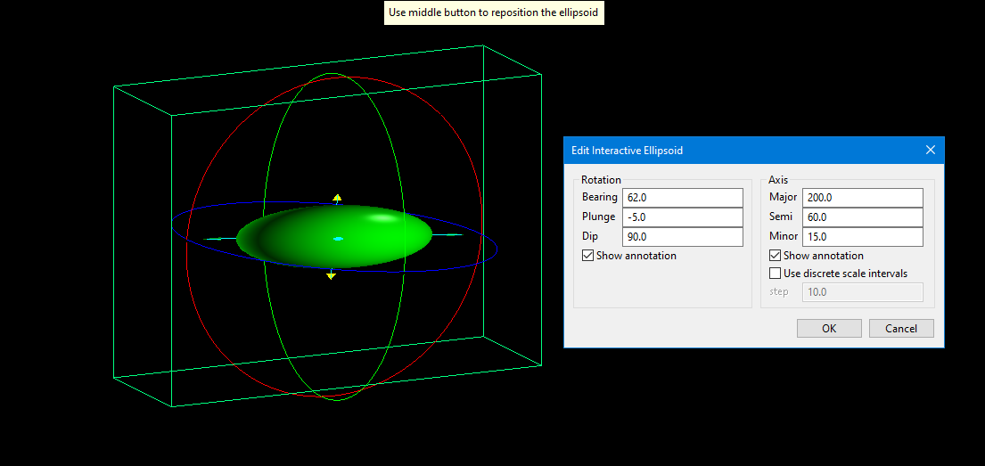
Click the Interactive button to adjust the search distances and orientation visually.
-
Set the origin by selecting a location on the screen. This point is an arbitrary point used to define the starting location for measuring the distance and orientation.
-
Set the parameters for rotation by adjusting the Bearing, Plunge, and Dip. Set the parameters for the distances by adjusting the Major, Semi, and Minor settings. You can do this by entering the numbers manually, or by clicking and dragging the arrows and rings on the screen.
-
Select Show annotations to toggle the display for showing the arrows.
-
Select Use discrete scale intervals to limit increasing or decreasing the distances by the Step size you enter.
-
Click OK to return to the main panel.
-
Variogram
Follow these steps:
-
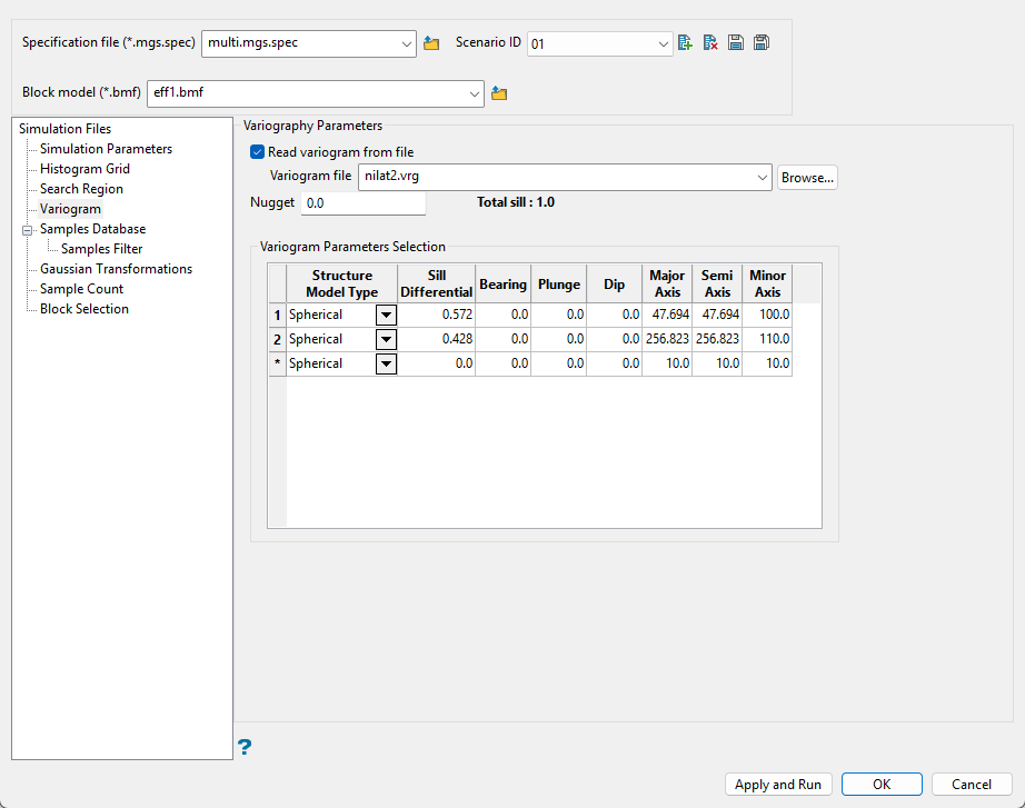
Select Read variogram from a file to use an existing variogram model. Use the drop-down list to select the model. Variogram models are stored in (
.vrg) files. -
Enter the nugget.
-
Select the type of model from the drop-down list labelled Structure Model Type.
The variogram model type can be one of the following:
Spherical
This type is the most commonly used for ore deposits. They exhibit linear behaviour at and near the origin then rise rapidly and gradually curve off.
Exponential
This type is associated with an infinite range of influence.
The sill is reached at the specified range parameter. In release 3.2 and earlier, users were required to enter a range parameter of one-third the practical sill range. To use this model, enter the practical distance of the sill as a range parameter. For backward compatibility, see the Exponential Model 3.
Gaussian
This type exhibits parabolic behaviour at the origin and, like the spherical model, rises rapidly. The Gaussian type reaches its sill smoothly, which is different from the spherical model, which reaches the sill with a definite break. The Gaussian model is rarely used in mineral deposits of any kind. It is used most often for values that exhibit high continuity.
In release 3.2 and earlier, users were required to enter a sill range of 3 times the actual sill range. To use this model, enter the effective range of the sill. For backward compatibility, see the Gaussian model 3.
Linear
This type is a straight line with a slope angle defining the degree of continuity.
De-Wijsian
This type is a representation of a linear semi-variogram versus its logarithmic distance.
Power
This type is computed as M - d**p where M = the maximum correlation defined as 1000.0, d = distance from the origin, p = model power. For this model type only the power p is the major axis radius. Adjust the size of the ellipsoid so that the major axis is the desired power. The size of the ellipsoid for this model does not change the calculation of the variogram.
Exponential Model 3
This is an un-normalised exponential model for compatibility with release 3.2 and earlier. This variogram will have the practical sill at three times the distance entered as range parameter.
Periodic
This is a sine wave with one complete period over the effective range. This model is not commonly used because it can cause samples at greater distances to have higher correlation.
Gaussian Model 3
This is an un-normalised Gaussian model for compatibility with release 3.2 and earlier. The input radius must be the effective radius multiplied by 3.
Dampened Hole Effect
Dampening is achieved by multiplying the covariance function by an exponential covariance, that acts as a dampening function.
-
Enter the Sill Differential. This represents the difference between the value of the variogram where it levels off and the nugget. For example, if you have a total sill of 1.0, and a nugget of 0.15, you want your sill differential to be 0.85 = (1.0 - 0.15).
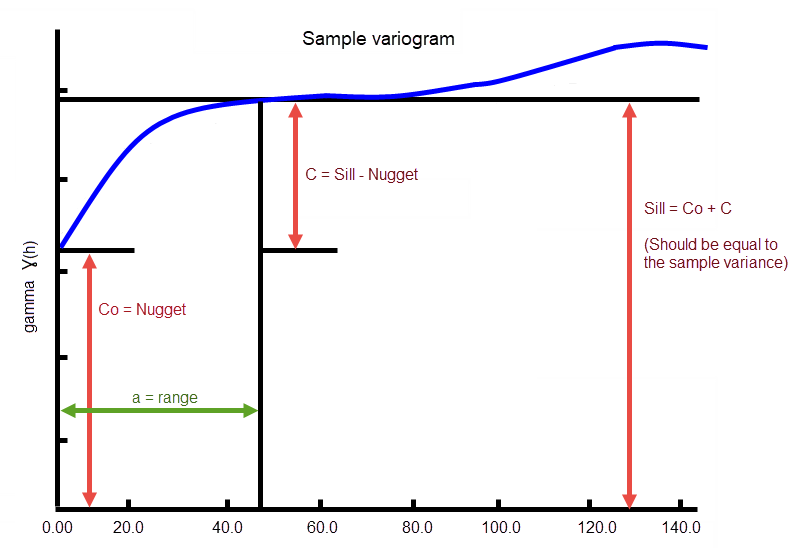
In the diagram, C0 is the nugget, and C is the sill differential.
-
Enter the Bearing (Rotation about the Z axis), Plunge (rotation about the Y axis), and Dip (rotation about the X axis) of the variogram.
-
Enter the radii of the Major, Semi, and Minor axes of the variogram.
Samples Database
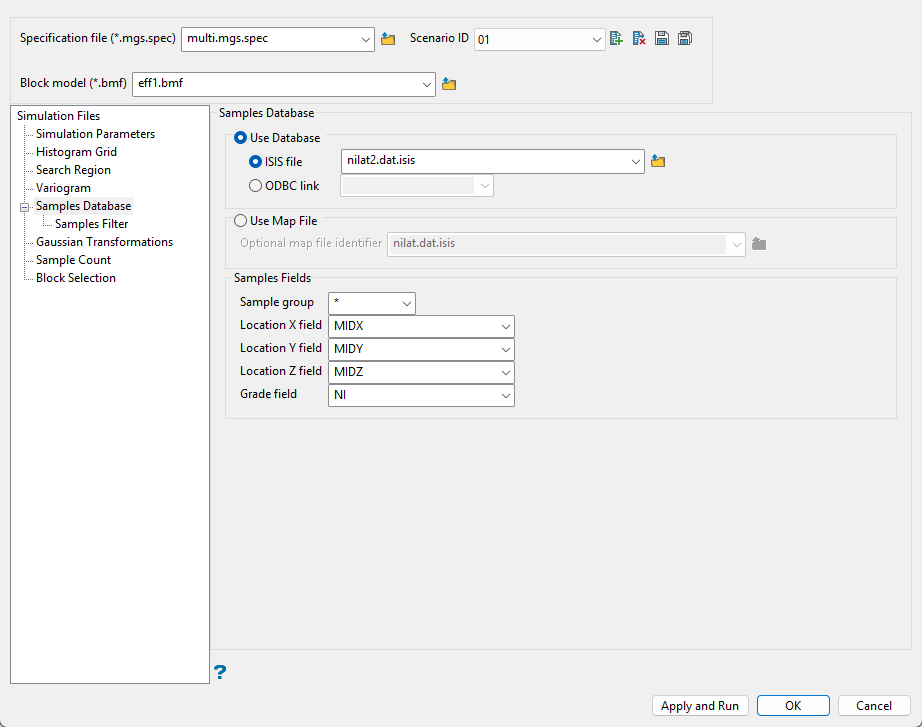
Use this pane to define the source of your samples. You can use an Isis database or a map file.
Follow these steps:
-
Select either a database or map file as your sample source.
-
To select a database, enable the option ISIS file, then select the file from the drop-down list. Click folder icon to select a file from another location.
You can also select an ODBC link for database files found on site servers.
-
To select a map file, enable the option labelled Use Map File, then select the file from the drop-down list. Click the Browse button to select a file from another location.
-
-
Map the correct fields by filling out the Samples Fields information.
-
Sample group - Enter the name of the groups (database keys) to be loaded in the field. Wildcards (* multi-character wildcard and % single character wildcard) may be used to select multiple groups. Multiple groups only apply to Isis databases (ASCII map files consist of one group).
-
Select the names of the fields containing the X, Y, and Z coordinates in the Location fields.
-
Select the name for the variable containing the Grade values.
-
Samples Filter
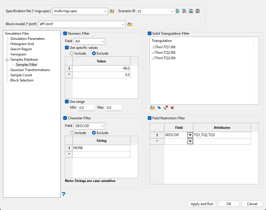
Use this panel to filter your sample data by setting restrictions on samples values, triangulations used, character values within database fields, and field attributes. You can use any combination of the four filters, or not use any at all. This panel is optional.
The example above shows one possible way to filter data. The filters will ignore all default assay values of -99.0, include only samples that fall within the three vein triangulations, ignore any sample that has a GEOCOD string equal to "NONE", and include samples that have an attribute label of TQ1, TQ2, or TQ3.
The following steps show how to set your filters.
-
Select the Numeric Filter checkbox to apply numeric restrictions to any field you select from the Field drop-down list. You can use specific values, a range of values, or both.
Note: Only numeric fields will be shown in the drop-down list.
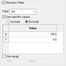
-
Select the option Use specific values to include or exclude whatever values you list under Values in the grid.
-
To use a range of values, select Use range, then enter the minimum and maximum values.
The range below is evaluated as
0.001 ≤ VALUE < 99999.0.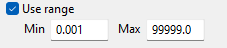
Select the Solid Triangulation Filter checkbox to limit the data by triangulation.

-
Clicking the Browse icon will display the following panel. From here you can select your triangulations. All triangulations found in the current working directory will be listed in the selection panel that will be displayed.
-
Selecting images from the panel
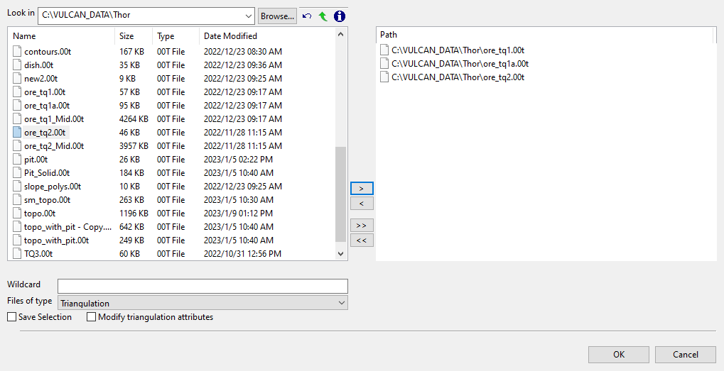
Click the Browse button to search for any triangulation not found in your current working directory.
Click on the name of the file(s) you want to select. Use the
 icons to go to the last folder visited, go up one level, or change the way details are viewed in the window.
To highlight multiple files that are adjacent to each other in the list, hold down the Shift key and click the first and last file names in that section of the list.
To highlight multiple non-adjacent files, hold down the CTRL key while you click the file names.
Move the items to the selection list on the right side of the panel.
- Click the
 button to move the highlighted items to the selection list on the right.
 - Click the
 button to remove the highlighted items from the selection list on the right.
 - Click the
 button to move all items to the selection list on the right.
 - Click the
 button to remove all items from the selection list on the right.
- Click the
-
Wildcard characters can be used to limit what appears on the list. Use an * for multiple characters or a % to replace a single character.
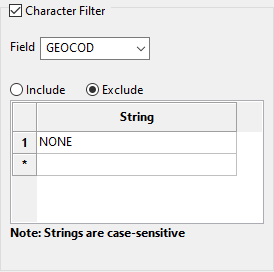
Select the Character Filter checkbox to limit the data by a character string found in the selected database field.
-
Select the database field from the Field drop-down list. Only character fields will be listed.
-
Decide whether you want to include or exclude the text string.
Important: The text strings are case sensitive and must be entered exactly as they will be found in the database.
-
Enter the string without quotation marks in the space provided. You can have multiple strings.
In the image above, our database is populated with four GEOCOD values: TQ1, TQ2, TQ3, and NONE. We have opted to include all values except those samples which have a value as NONE. Any sample that contains a GEOCOD value of NONE will be excluded from our sample population.
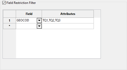
Select the Field Restriction Filter checkbox to restrict the data by field attribute.
-
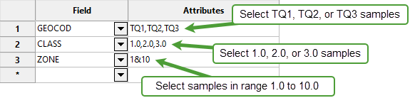
Select a Field from the drop-down list and enter applicable selection criteria to filter the samples by in the Attributes column.
Include spaces in the entries in the Attributes column only if spaces are included in the desired field values.
When entering a range, always enter the smallest number specified before the largest number.
-792&-720since-792is smaller than-720. This range is evaluated as-792.0 ≤ VALUE < -720.0.
Gaussian Transformations
![]()
-
Select the transform file from the drop-down list, or click the Browse button to select a file in a location other than the top level of your current working directory.
You will need to use an existing transformation file generated by any of the following methods:
Normal Score - Use the Normal Score option to transform data from any distribution so that the transformed values follow a standard (normal) Gaussian distribution. The transformation is performed using the quantile transformation with a target distribution being a Gaussian standard.
BM Normal Score - Use the BM Normal Score option to transform block model data from any distribution so that the transformed values follow a standard (normal) Gaussian distribution. The transformation is performed using the quantile transformation with a target distribution being a Gaussian standard.
Stepwise Gaussian - Use the Stepwise Gaussian option to transform two or three database variables such that the bivariate (or trivariate) and marginal distributions of the transformed variables are all standard Gaussian.
BM Stepwise Gaussian - Use the BM Stepwise Gaussian option to transform two or three block model variables such that the bivariate (or trivariate) and marginal distributions of the transformed variables are all standard Gaussian.
Normal Score Back - Use the Normal Score Back option to use an existing Normal Scores transformation lookup table and transform the block model values that are in Gaussian units back to the original grade units.
Sample Counts
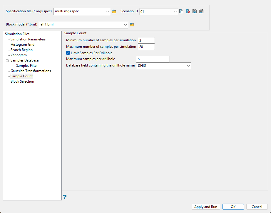
Use this pane to determine how many samples you want to use during the calculation of each block.
Follow these steps:
-
Enter the Minimum number of samples per estimate that have to be found to generate an estimate. Blocks with less than this number of samples within the search ellipsoid or box are assigned the default grade value.
-
Enter the Maximum number of samples per estimate to be used in any grade estimation. For example, the estimation program may find 30 samples near a block centre. If you had specified a maximum of 10 samples, then only the 10 samples closest to the block centre are used. The distance to the block centre is calculated by an anisotropic distance based on the search radii. Up to 999 samples per estimate are allowed.
-
Select Limit Samples Per Drillhole to limit the number of samples to use that come from a single drillhole.
If you enable this option, you will need to enter the Maximum samples per drillhole that are allowed to come from a single drillhole.
-
Select the Database field containing the drillhole name. This is the name of the field that contains the drillhole name. This list draws from is the database selected in the Samples Database pane.
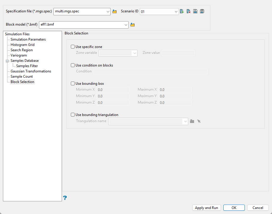
Block Selection
-
Select which blocks you want to include in the simulation run. By default, all blocks will be included unless otherwise specified.
Use specific zone
You will need to specify the variable, as well as a particular value.
Example: If you have a variable called
Materialin your block model and want to restrict blocks to those where the material equals ore, selectMaterialas the variable and enteroreas the value.Use test condition on blocks
You can limit the blocks by adding a condition on a numeric block model variable.
Example: To select blocks where iron has a value greater than 10.0, the condition would be
Fe GT 10.0The maximum size of the condition is 256 alphanumeric characters. Refer to Appendix B of the Core Appendices for a full list of available operators and functions.
Use bounding box.
If you select this option, you must enter the minimum and maximum coordinates for X, Y, and Z in the block model coordinates (X, Y, Z CENTRE). If the block model origin is set at 0,0,0, then real world coordinates should be entered in the X, Y, and Z minimum and maximum coordinates. If the block model origin is set at real world coordinates, then enter coordinates for the bounding box that are offset a certain distance from the origin. The distance of offset will be determined by the dimensions of your bounding box. It will be the distance to the minimum and the distance to the maximum X, Y, and Z from the origin of the block model.
Use bounding triangulation
This is useful when you want to evaluate reserves in a particular solid triangulation, such as a stope.
Select the triangulation from the drop-down list. or click the Browse icon to select one from a location other than the top level of your current working directory.
Tip: To use all blocks outside of the selected triangulation, select the Reverse selection option in addition to the bounding triangulation.
-
Click Apply and Run to begin the simulation.
Click OK to save your settings and exit without running the simulation.
Click Cancel to exit without saving.
