Steep Horizon Modeller
This option enables the creation of surfaces, solids, and block models using various modeling methods. Models are generated directly from drillhole, composite, or design databases.
Additionally, horizon data points from the input database can be saved into specified layers. This tool also supports the use of relimiting polygons to include or exclude specific areas from the output triangulations.
Input
The input data can be sourced from drillhole databases, composite databases, or CAD data from design databases.
Output
The output will be a set of surface or solid triangulations for each horizon selected. A block model can also be created with the horizon name assigned to a block model variable and the horizon solids assigned to the boundaries.
In the Streamlined Stratigraphy tool, once you confirm that the deposit dips more than 30 degrees, the workflow will guide you to the Steep Horizon Modeller panel. The panel is divided into nine tabs:
Data Reliability
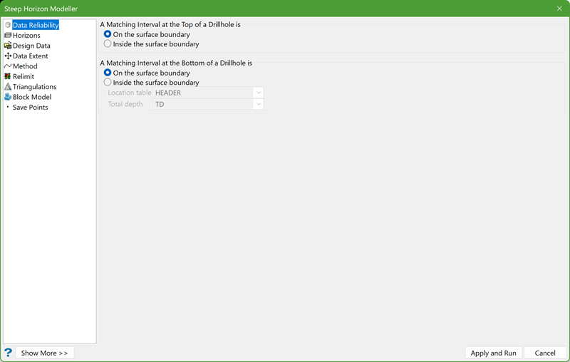
A Matching Interval at the Top of a Drillhole is
- On the surface boundary - Select this option to ensure that the interval starting at depth 0 is reliable. If it is reliable, then the horizon model value at this location honours the input data.
- Inside the surface boundary - If this option is selected, the modeller assumes that the horizon model value cannot be interpolated lower down the depth but can be interpolated higher.
A Matching Interval at the Bottom of a Drillhole is
- On the surface boundary - Select this option to ensure that the interval ending at total depth is reliable. If it is reliable, then the horizon model value at this location honours the input data.
- Inside the surface boundary - If this option is selected, the modeller assumes that the horizon model value cannot be interpolated further up the total depth but can be interpolated lower. Provide the Location table and Total depth values for interpolation.
Horizons
This section allows the selection of modelling horizons.
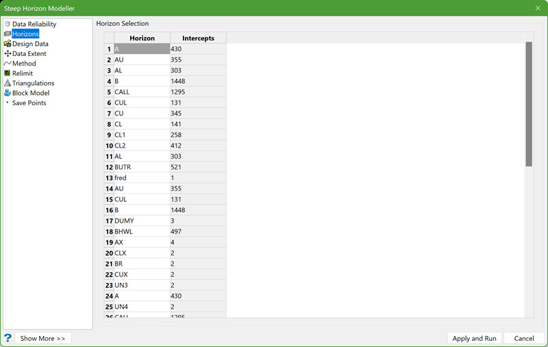
There is a set of controls on the right to list the horizons and their respective intercepts.
Note: The order of the horizons is important. They should be specified in an order perpendicular to the modelling plane - hanging wall to footwall.
The horizon list can be specified by:
1. Manually typing in the values in the Horizon column.
2. Clicking the button to load all the horizons from the specified database automatically. The intercept count will also be displayed in the Intercepts column.
There are a few controls to help with the selection.

|
Load all the horizons from the input drillhole and composite database. Note: This button is enabled only if there is a drillhole or composite database selected. |

|
Update the count of the intercepts for each horizon from the input drillhole and composite database. Note: This button is enabled only if there is a drillhole or composite database selected. |

|
Select all the horizons. |

|
Deselect all the horizons. |
|
|
Reverse the order of horizons. |
|
|
Move the horizon(s) one row up. |
|
|
Move the horizon(s) one row down. |


Note: To select the horizons, check the box at the front of each row. To move the horizons up/down, one or more rows need to be selected.
Design Data
This section allows the input of CAD data from a design database.
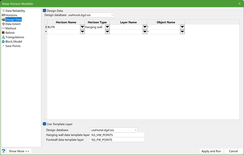
Design Data
Select this checkbox to use pre-existing design data when creating surface models.
Horizon Name
Type in the horizon name or select from the drop-down list. Enter * to select all the horizons.
Horizon Type
Specify whether the data is used to model hanging wall or footwall.
Layer Name
Specify the design layer name which contains the CAD data.
Object Name
Choose the object name or enter * for all the objects.
Use Template Layer
Select this check box to use pre-defined names of layers for the selected horizons. Choose a design database and enter the hanging wall and footwall data template layers.
Note: The default value for the hanging wall data is %S_HW_POINTS and the footwall data is %S_FW_POINTS, which is as same as the default template in Save Points.
Data Extent
This section allows the user to manually or dynamically specify horizon data plane and extent.
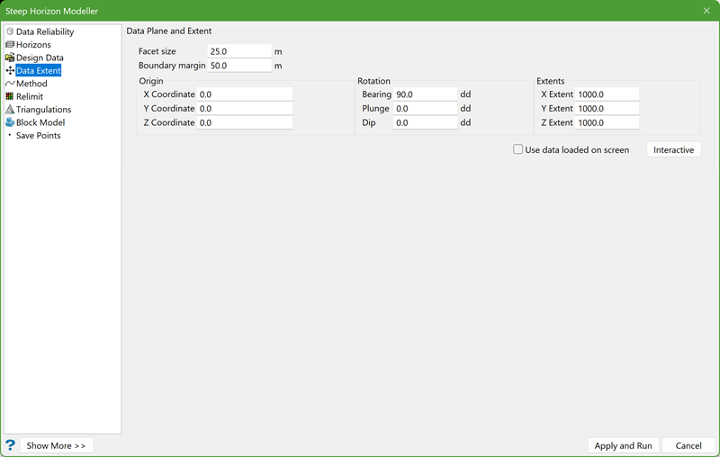
Facet size
This is the resolution of the triangle facets in the resultant model. If this value is changed, the values of X, Y, and Z extents will also change. The extent value will be rounded to the nearest divisible value of the facet size. The unit of the facet size is same as specified in the .dg1 file.
Boundary margin
This is a buffer distance applied to the outermost horizon data to be modelled. It adds to the X Extent, Y Extent and Z Extent, which is applied when the Interactive button is clicked. The unit of the boundary margin is same as specified in the .dg1 file.
Interactive
Use data loaded on screen
If this option is unchecked and the Interactive button is clicked, the modeller tool analyses the specified input data source including the data from drillhole, composite, and design databases, and fetches all the data of the selected horizons, figures out the best model plane and displays the 3D extent to include those data. The information of the extent’s origin point and bearing, plunge and dip, and the X, Y, Z extent sizes are calculated and displayed in the Edit Interactive Data Extent panel shown below.
If this option is checked and Interactive button is clicked, the modeller tool uses the data loaded on the screen and performs the same calculation of the extents and displays information in the interactive panel.
After the calculation, the Edit Interactive Data Extent panel pops up displaying the calculated information. Also, a 3D extent box is displayed on the screen.
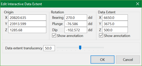
The calculated information can be changed by typing in the desired values or by using the 3D extent box.
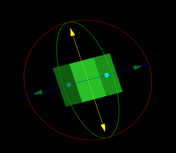
Figure 1 - 3D extent box
Use 3D extent box to make adjustments to:
- The location of the model by holding down the centre button of the mouse and dragging the model to the desired position.
- The dimension by hovering over one of the arrow tips until the cursor changes to a PLUS symbol, then holding down the left button of the mouse and dragging back and forth to resize.
- The model rotation by hovering the mouse over one of the spherical rings until the cursor changes to a CIRCLE, then holding down the left button of the mouse and dragging back and forth to change the rotation.
When all adjustments have been made, click OK to save the changes and return to the main panel or Cancel to discard the changes.
Note: If X, Y and Z extent values are manually changed or modified via the Edit Interactive Data Extent panel, it will be automatically rounded to the nearest value divisible by the facet size.
For definition of Origin, Rotation, and Extent fields, please refer to the Block Model.
Method
This section allows the selection of horizon modelling methods and parameters.
There are two methods available when creating multiple horizon models:
- Structural Surfaces
- Stacking
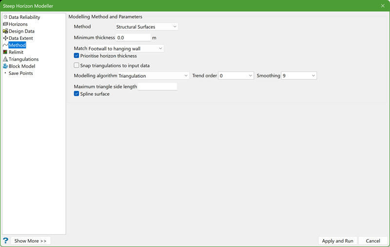
Structural Surfaces Method
This method models individual hanging wall and footwall for each horizon.
In the above example, a triangulation method is used with a 2nd order trend and 9 Smoothing passes. To avoid very long triangle edges, the Maximum triangle side length is limited to 5000.
Note: The Maximum triangle side length field appears on the panel because the Triangulation Modelling algorithm is chosen. Each modelling algorithm has its own required parameters. Selecting different algorithms will populate the panel with unique fields.
Match
Should a horizon cross its neighbour, either the footwall is forced to the hanging wall position or the hanging wall is forced to the footwall position. Control this selection from the drop-down list.
Prioritise horizon thickness
Check this option to maintain the horizon thickness while matching between multiple horizons.
Snap triangulations to input data
Check this option to have the triangulation snapped to the input data points. This option is available for both modelling methods.
Stacking Method
This method creates all horizon models based on one selected structural surface. The selected surface becomes a reference for creating the rest of the models. The remaining surfaces are created by adding and subtracting thickness and mid-horizons from the reference surface.
When selecting the Stacking Method, define Modelling algorithms for both the Reference Horizon and the Thickness models.
Reference Horizon
The reference horizon can be selected from the Horizon drop-down list, and is generally the horizon with the most reliable data.
Thickness
It is possible to use a different algorithm when modelling Thickness models.
Note: Each modelling algorithm has its own required parameters. Selecting different algorithms will populate the panel with unique fields.
Relimit
This section allows the output surface triangulations to be relimited by polygons and data extent.
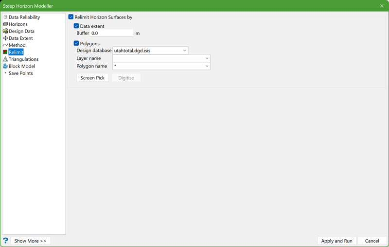
Relimit Horizon Surface by
Select this option to relimit the output surface triangulations by one or more specified polygons.
Data extent
Select this option to relimit the surface triangulations by its data extent.
Buffer - Define a distance to extend the data extent for relimiting.
Polygons
Define the polygons using the drop-down selections, or click Screen Pick to select one or more polygons loaded on the screen.
If the Design database and Layer name are specified, the Digitise button is enabled and allows digitising one or more polygons on screen.
If the layer name already exists, a dialog box is displayed confirming whether to append, replace or cancel.
Note: Clockwise polygons include triangles which fall inside the extent view projection of polygon extents defined in Data Extent.
Anti-clockwise polygons include triangles which fall outside the extent view projection of polygon extents, also defined in Data Extent.
Triangulations
This section allows user to specify the name, location, and attributes of the output triangulations.
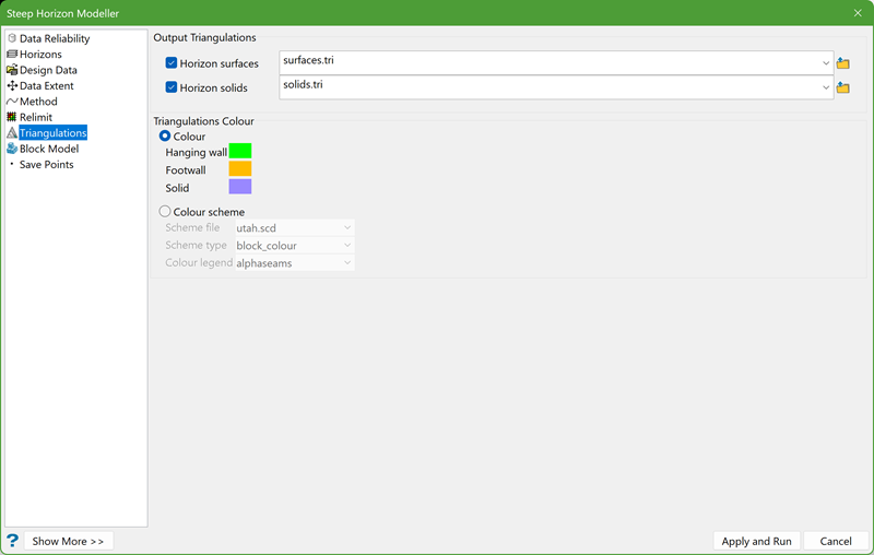
Output Triangulations
Horizon surfaces
Select this option to specify the output folder for the surface triangulations modelled. This will also enable the Save Points section. The default folder is surface.tri residing in the current working directory. Browse to choose another location.
Note: The output surface triangulations are named with the convention <proj><horizon>.hwt for hanging wall or <proj><horizon>.fwt for footwall, where <proj> is the project prefix and <horizon> matches what is defined in the Horizons.
Horizon solids
Select this option to specify the output folder for the triangulation solids modelled. The default folder is solids.tri residing in the current working directory. Browse to choose another location.
Note: The output solid triangulations are named with the convention <proj><horizon>.00t, where <proj> is the project prefix and <horizon> matches what is defined in the Horizons.
Triangulations Colour
There are two options to add colour to the output surface and solid triangulations:
Colour
Select this option for the output surface and solid triangulations to be a single colour. Assign different colours for hanging wall, footwall, and solid triangulations. The colours used for the triangulations will be selected from the current colour table.
Colour scheme
Select this option to use a Vulcan colour scheme to colour the output surface and solid triangulations. Select the scheme file and colour legend from the drop-down lists.
Delete temporary files on completion
This option is turned on by default, which deletes all temporary files created during the modelling process.
Block Model
This section allows creating a block model from the input data.
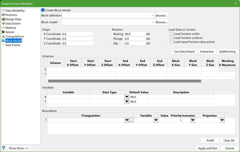
Create Block Model
Select this option to create a block model from solid triangulations.
Block definition
Enter or select from the drop-down list, the name of the block model definition file. The naming convention is <name>.bdf.
Block model
Enter the block model identifier (<bfi>) of the block model. The maximum size of the identifier is 20 alphanumeric characters. The file extension (.bmf) is automatically added.
Note: Use an alphabet as the first character of the block model identifier.
Origin
X/Y/Z Coordinate
The origin point is an arbitrary point used to define the start of the offsets in the scheme and the pivot for the rotations. The origin point, offsets, and rotations are used in conjunction with the Parent scheme to define the position of the block model in space.
Rotation
Bearing
Enter the bearing of the X axis around the Z axis.
When the X axis is at 0 degrees, it is pointing due North. By default, the bearing for block models are oriented at 90.0°. The bearing angle can be determined by using the Analyse>Details>Distance option, which displays bearing as well as the distance.
Plunge
Enter the plunge of the ore body in the ZY plane.
The plunge angle can be determined by following the steps given:
- On the screen, rotate the ore body in the plane until the plunge angle can clearly be seen.
- Construct a line parallel to this direction.
- Use the Analyse>Details >Full option to display an inclination that is very close to the plunge angle.
Dip
Enter the dip of the ore body in the ZX plane. The dip angle can be determined in a similar manner to the plunge.
Note: Both the plunge and dip angle, as well as the origin point, may need adjustments to contain the ore body in the block model extent.
Interactive
Click Interactive button to create the extents of the block model interactively on the screen.
Steps:
- Begin by clicking on the screen where the origin of the model is to be located. A generic block model will be created whose size and position can be adjusted.
- Make adjustments to the location of the model by holding down the centre button of the mouse and dragging the model to the desired position.
- Make adjustments in dimension by hovering over one of the arrow tips until the cursor changes to a PLUS symbol, then hold down the left button of the mouse and drag back and forth to resize.
- Make adjustments in the model rotation by hovering the mouse over one of the spherical rings until the cursor changes to a CIRCLE symbol, then hold down the left button of the mouse and drag back and forth to change the rotation.
When the Interactive button is clicked, the Edit Interactive Block Model panel is displayed. As changes are made interactively on the screen, they will be reflected on this panel.
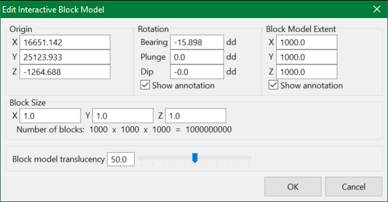
When all adjustments have been made, click OK to save the changes and return to the main panel or click Cancel to discard the changes.
Use Data Extent
Click this button to load the data extent defined in Data Extent.
Subblocking
Click this button to prefill the suggested subblocking information defined in the Schemes.
Load Data on Screen
Load horizon solids/Load horizon surfaces
On entering the Interactive mode, the initial block model extent will be automatically adjusted to the extents of the triangulations and design objects loaded on the screen.
The triangulations already loaded on the screen are replaced by the most recent.
Load saved horizon data points
Select this option to load previously saved data points and design data to be used by the Interactive mode.
The data is loaded automatically from the hw/fw data points dgd layers and displayed on the screen. Previously loaded data points are replaced by the latest layer content.
Schemes
This section allows to define the blocking constraints for a model. A scheme is a list of specifications for the extent of the blocks and their sizes. By default, there must be a Parent scheme which contains a parent cell size that defines the maximum cell size over the domain of the model. The parent cell size partitions all of the volume in the model. Only one parent cell volume can be specified at a time.
Subblocking splits a parent cell into smaller cells that better model the geometry of the geological boundaries. One can specify a number of subblocking schemes geographically i.e. different coordinate ranges can have different subblocking cell sizes.
If the parent cell size is 10 × 10 × 10 (in X, Y, and Z directions) and you choose a sub-cell size of 2 × 5 × 5, then the parent cell is split to create the minimum number of cells required to represent that geometry from the smallest cells available (the sub-cell size must be divided evenly into the parent cell size). This means that the blocks are coalesced with the boundary. The result is an optimum number of sub-cells with an equivalent definition to that would exist had every sub-cell been split/created.
Note: The first row in this table is always used to define the parent scheme, with subsequent rows being used to define the sub-block areas.
Defining parent scheme
- Scheme - Enter the name of the parent scheme.
- Offsets - Enter the start and end X/Y/Z offset distances. These distances are relative to the origin point defined previously in the Origin section. If you require a model over the full area of the ore body, then the offset distances must include all triangulations that define the lithology of the ore body. Models can be made over portions of the ore body area by restricting the offsets.
- Block X/Y/Z Size - Enter the minimum cell size.
- Blocking X/Y/Z Maximum - These columns are not applicable to the parent scheme.
Variables
Enter the name of the variable (a maximum of 30 alphanumeric characters) for block model.
Boundaries
Boundaries define whether a variable value occurs inside or outside, above or below the nominated triangulations.
For more details, please refer to Block>Construction>New Definition.
Prefill
Click this button to get the horizon field as a variable and the output solid triangulations as the boundaries.
Clear All
Click this button to clear the contents in Variables and Boundaries.
Save Points
This section allows users to save the generated horizon data points into specified layers.
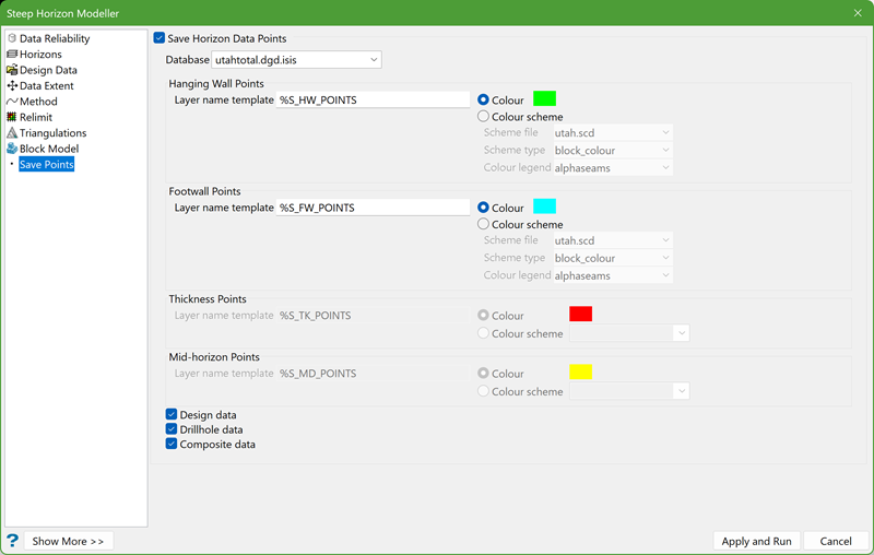
This section is enabled only if the Horizon Surfaces option in the Triangulations section is selected.
Save Horizon Data Points
Select this option if you want to save the input data as design data points into the specified layers.
Database
Choose the database in which the resulting data points will be generated.
Hanging Wall Points/Footwall Points
The Layer name template defines the name of layers where the resultant points will be saved. The panel default is %S_HW_POINTS, where %S is automatically replaced by the necessary horizon name as defined in the horizon list and _HW_POINTS is a fixed suffix assigned to the horizon name for hanging wall points.
Similarly, the panel default for Layer name template is %S_FW_POINTS for footwall points.
Thickness Points/Mid-horizon Points
When choosing the Stacking method in the Method section, the options to save thickness points or mid-horizon points are enabled. The thickness points represent the horizon thickness and the mid-horizon points represent the value between the continuous horizons defined in the horizon list.
The panel default for the Layer name template is %S_TK_POINTS for Thickness Points and %S_MD_POINTS for Mid-horizon Points.
For all of the four points, there are two types of colouring options:
ColourSelect this option for the resulting points to be single coloured. The colours used for the saved points will be selected from the current colour table.
Colour scheme
Select this option for the Vulcan colour scheme to colour the resulting data points.
For hanging wall and footwall points, select the scheme file, type, and colour legend from the respective drop-down lists.
For thickness and mid-horizon points, choose a colour scheme. You don't need to specify colour legend as it comes from the CONTOUR scheme.
Input data
Specify the input data to be saved by selecting one or more of the three databases namely, Design, Drillhole, and Composite.
